Chapter 21 The Uniform Distribution
21.1 Introduction
We have learned about important discrete random variables such as the binomial and about important continuous random variables such as the normal. In this chapter we add to our repertoire some other useful distributions including the geometric, negative binomial, and poisson discrete random variables and the uniform and exponential continuous random variables.
21.2 Chapter Scenario - Lovin’ the Airport
Suppose a domestic flight leaves at 5:00pm and has 50 passengers who show up independently at the airport at uniformly random times between 3:15pm and 4:30pm. How many passengers can we expect to have arrived at the airport by 4:00pm, one hour before takeoff? How confident can we be in this answer?
21.3 The Uniform Distribution
The uniform random variable is a continuous random variable that is equally likely along its entire range of possible values. Like the normal distribution, the area under the curve between two values is the probability of the random variable being in the interval but unlike the normal bell-shaped curve, the uniform probability density function is a flat, horizontal line. If the uniform random variable X ranges from a minimum of \(a\) to a maximum of \(b\), we abbreviate this \(X \sim UNIF(a,b)\).
21.3.1 The Uniform Probability Density Function
The uniform probability density function is flat and the area under the curve equals the probability. For X, a uniformly distributed random variable with a minimum of a and a maximum of b, \(X \sim UNIF(a,b)\), so that the total area under the curve is 1, the height of the curve must be \(1/(b-a)\) between a and b and 0 elsewhere. The code below creates a function to plot different uniform random variables
uniform_Plot <- function(a, b){
  xvals <- data.frame(x = c(a, b)) #Range for x-values
  ggplot(data.frame(x = xvals),aes(x = x)) + xlim(c(a, b)) +
    ylim(0, 1/(b - a)) +
    stat_function(fun=dunif, args=list(min=a, max=b), geom = "area",
                  fill="green", alpha=0.35) +
    stat_function(fun = dunif, args = list(min = a, max = b)) +
    labs(x="\n u", y="f(u) \n",
         title=paste0("Uniform Distribution \n With Min = ", a, " & Max = ", b, " \n")) +
    theme(plot.title=element_text(hjust = 0.5),
          axis.title.x=element_text(face="bold", color="blue", size=12),
          axis.title.y=element_text(face="bold", color="blue", size=12)) +
    geom_vline(xintercept=a, linetype="dashed", color="red") +
    geom_vline(xintercept=b, linetype="dashed", color="red")
}
Source: http://dkmathstats.com/plotting-uniform-distributions-in-r-with-ggplot2/
Here is the plot of UNIF(4,12).
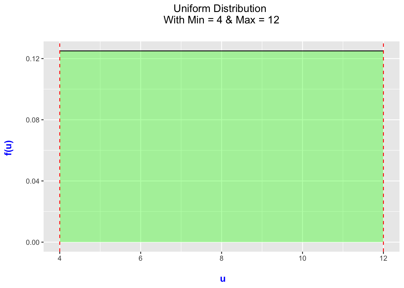
For uniform random variable \(X \sim UNIF(a,b)\), the expectation is \(E(X)=\frac{a+b}{2}\) and the variance is \(Var(X)=\frac{(b-a)^{2}}{12}\) and standard deviation \(SD(X)=\sqrt{\frac{(b-a)^{2}}{12}}\).
21.3.2 The Uniform Random Variable in R
For X a uniform random variable we use the following. Since by default min=0 and max=1, for X that is uniformly distributed between a and b, \(X \sim UNIF(a,b)\), we must replace 0 and 1 by a and b, respectively.
To find the probability of X being less than q, \(P(X < q)\), use punif(q, min = 0, max = 1, lower.tail = TRUE).
To find the probability of X being greater than q, \(P(X > q)\), use punif(q, min = 0, max = 1, lower.tail = FALSE) or 1-punif(q, min = 0, max = 1, lower.tail = TRUE).
To find the inverse probability, that is the value of x such that \(P(X \leq x) = p\) use qunif(p, min = 0, max = 1, lower.tail = TRUE).
To generate a random sample of size n from a uniform random variable use runif(n, min = 0, max = 1).
21.3.3 Example - The UNIF(0,1) Random Variable
The basis for most random number generator schemes is a uniform random variable X with a minimum of 0 and a maximum of 1, \(X \sim UNIF(0,1)\). The probability density function is visualized below.

Because the default min=0 and max=1 we could leave these parameters out when using punif(), qunif(), or runif(). For example, we can use runif(n) to generate a sample of size n. Here is a sample of twenty random UNIF(0,1):
##  [1] 0.33615347 0.46372327 0.06058539 0.19743361 0.47431419 0.30104860
##  [7] 0.60675886 0.13001210 0.95865471 0.54684949 0.39561597 0.66453861
## [13] 0.98211229 0.67821539 0.80602781 0.63417988 0.27073646 0.55290413
## [19] 0.73795568 0.82840038
Variations on UNIF(0,1) is how other random numbers are generated. Watch what happens when we multiply runif(n=20) by 4.
##  [1] 1.0404032 2.2734415 0.6059931 0.3797474 3.0476664 2.1437142 1.3115237
##  [8] 3.6974241 2.3932470 0.2585466 0.5654715 3.4503960 0.1353209 1.9608193
## [15] 2.0247205 3.0481376 0.1842237 0.2086938 2.3240237 0.7005295
In this case, we stretched the range so that the values are now UNIF(0,4).
Suppose in addition to stretching by a factor of 4 we subtract 2.
##  [1]  1.58744205  1.09188645  0.39513140  0.39698649  0.40748783 -1.98852087
##  [7]  1.85165059 -1.72359197 -1.55484713  1.09709086 -0.37952902 -1.16007461
## [13] -1.42049234  1.05396454  0.65016560  1.86619209 -0.42715126  0.41739040
## [19] -0.94499729 -0.04212705
This generates random uniform numbers UNIF(-2,2).
And if we had added 2 instead:
##  [1] 3.638652 3.402199 5.522949 2.457047 3.580058 2.035257 4.805197 4.583177
##  [9] 2.153902 4.163981 3.248564 2.912225 5.683229 2.258957 2.564514 3.941337
## [17] 4.460030 3.103937 3.672544 2.375969
Now we are generating random uniform numbers UNIF(2,6).
Of course, we could generate all of these directly using runif(0,4), runif(-2,2), and runif(2,6) but now we know a little more about how R does it under the hood.
21.3.4 Example - Catch a Flight
Suppose that the time check in at the airport for a 5:00pm flight is uniformly distributed from 3:15pm to 4:30pm. If we let X represent the amount of time in minutes after 3:15pm that a person shows up then \(X \sim UNIF(0,75)\).
To find the probability a person chosen at random shows up before 4:15pm:
## [1] 0.8To find the probability a person chosen at random shows up after 4:15pm we have options:
## [1] 0.2## [1] 0.2To find the 66th percentile, that is the amount of time after 3:15pm that \(66\%\) of people show up:
## [1] 49.5As a time, this would translate into 3:15pm plus 49.5 minutes which would be 4:04:30pm.
To generate a random sample of 50 passengers and the number of minutes after 3:15pm that they show up:
##  [1] 26.972408 55.429884  7.265998 29.899550 14.413928 68.177214 64.060610
##  [8]  7.276282 33.068926 23.091668 63.425941 11.603131 17.645577 74.495657
## [15] 16.354141 57.054788 20.117461 23.867858 70.933170 71.377694 20.883991
## [22] 26.735208 22.420707 30.888983 54.331459 24.139597  7.635658 17.286533
## [29] 31.518733 45.225700 50.675503  5.745529 13.120406 46.839767 74.761282
## [36] 29.505624 47.667820 49.922151 19.637350 30.995056 59.864449 29.439025
## [43] 54.155770 29.243570 42.564885 31.680140 24.824509 48.783081 35.102692
## [50] 55.207681
Doesn’t this give you a feeling of power? It would be easy for this go to our head.
21.4 Chapter Scenario Revisited - Lovin’ the Airport
Recall, a domestic flight leaves at 5:00pm, has 50 passengers who show up independently at uniformly random times between 3:15pm and 4:30pm and we want to know how many passengers we can expect to have arrived by 4:00pm and how confident can we be in this answer?
As we have seen, the time in minutes after 3:15pm that a passenger arrives can be modeled with a uniform random variable, \(X \sim UNIF(0,75)\).
The probability an individual passenger chosen at random will have arrived by 4:00pm is
## [1] 0.6We have 50 passengers and the probability any one of them arrives by 4:00pm is 0.6. The total number of passengers who have arrived by 4:00pm is thus like a binomial random variable with n=50 and p=0.6. The expected number of passengers to have arrived is 30 but this could vary. Check out this distribution:

##  [1] 0.003360382 0.007617426 0.016034764 0.031405553 0.057343761 0.097807364
##  [7] 0.156168331 0.233982953 0.329861684 0.438965068 0.553523621 0.664386736
## [13] 0.763124199 0.843909395 0.904498293 0.946044965 0.972011635 0.986749475
## [19] 0.994312314 0.997802855 0.999242703
While we expect around 30 there is only an 11.4558553 \(\%\) chance of exactly 30. This kind of knowledge could help us know how to more effectively manage airport traffic.
21.5 Exercises
21.5.1 Exercise - Transforming UNIF(0,1)
- Describe a transformation on
runif(0,1)that generates uniform random numbers with a min=0 and max=3. - Describe a transformation on
runif(0,1)that generates uniform random numbers with a min=-3 and max=3. - Describe a transformation on
runif(0,1)that generates uniform random numbers with a min=4 and max=12.
21.5.2 Exercise - Showing Up for Class
Suppose that in a class of 20 students that begins at 2:00pm, the time each student shows up is independent of other students and is uniformly distributed from 1:55pm to 2:10pm. (a) What is the probability a student chosen at random will arrive on time? (b) At what time can we be 90% certain a student chosen at random has arrived? (c) What is the probability student A shows up before student B? (d) What is the probability that a majority of students will show up on time?