Chapter 1 Probability Basics
1.1 Introduction
Probability is the measure of the likelihood of an event. In this chapter, basic terminology and principles of probability are introduced beginning. We begin with finding probabilities for simple events for such experiments as tossing a die and then examining how to handle compound events involving the logical NOT, AND, OR connectives. Then it gets exciting when we introduce conditional probability.
1.2 Chapter Scenario - The Three Card Game
There are three cards – one blue both sides, one red on both sides, and one blue on one side and red on the other. The cards are shuffled (both interspersed and randomly turned over) and you receive one of the three cards and it is placed face down on the table. You know only the face you see and not the color of the other side of the card. If the other side of the card is a different color, you win \(\$1\) while if the other side of the card is the same color you lose \(\$1\).
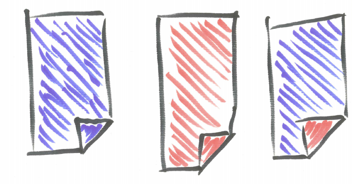
Figure 1.1: Three Card Game
What do you think the probability is that you will win? A fair game is one in which the payoffs and probabilities give neither you nor your opponent (often called the house) a systematic advantage. Does this game sound like a “fair” game to you? Explain.
1.3 Terminology
Before getting back to resolve the Three Card Game question, let’s develop some basic probability terminology.
A probability experiment is a process with a random element producing a well-defined outcome. Examples of a probability experiment are such as things as tossing a die or receiving the genes that determine one’s eye color. The probability of an event is the measure of the likelihood of that event on a scale of 0 to 1 where a probability of 1 can be interpreted as certainty the event will occur and a probability of 0 interpreted as certainty the event will NOT occur. There are two main schools of thought regarding what probability is - the frequentist and the bayesian - and the debate between these schools can be heated but for our initial purposes we will think of the probability of an event as the relative frequency of its occurrence in the long run. In very informal shorthand, we think of probability as the ratio of successes to the total number of trials as shown below.
\[Probability = \frac{successes}{total}\]
We must be careful to distinguish between exact theoretical probabilities and approximate empirical probabilities. Theoretical probability is exact and is based on assumptions about all the possible basic outcomes, often that they are equally likely. We use theoretical probability when it is reasonable to make assumptions like these about the probability experiment.
Empirical probability is approximate and is based on performing the probability experiment a number of times and examining the data. We use empirical probability when the situation is complex enough that theoretical approaches are not accessible and when data can be gathered. Both approaches, the theoretical and the empirical, have value and you will learn when and how to use each of them.
A third approach is subjective probability in which probability estimates are derived from personal judgments. This approach is used when theoretical and empirical approaches are not available like like for one-time events such as estimates of a certain bill passing congress. The use of subjective probability is also very powerful when combined with effective tools for updating probability estimates based on new information and evidence. These tools include Bayes’ Theorem and other techniques of bayesian statistics to be discusssed later in the text.
1.4 Example - Rolling a Die
Consider the probability experiment of rolling a die. We say it is a fair die if each of the six sides are equally likely. With this assumption, we can approach probability questions using theoretical probability. In this case, the probability of the die landing on any particular side is \(1/6\) which can also be approximated as \(0.167\) or \(16.7\%\). This means that as the experiment is repeated over and over again the proportion of the time the die lands on that particular side ultimately approaches \(frac{1}{6}\). Note, a probability equalling \(1/6\) does not mean that in any number of trials we will obtain that result exactly \(1/6\) of the time as samples will vary.
An empirical approach to the probability experiment of rolling a die would be to actually perform the experiment a large number of times and observe what happens. Running a simulation of rolling a fair die might be instructive here. The R code below performs 10,000 trials of rolling a die and recording the results in both a table and a histogram. At this point, focus on the output and don’t worry so much about the R code.
die <- sample(x=1:6, size=10000, replace = TRUE)
sim_die <- data.frame(die)
knitr::kable(table(sim_die),
  caption = 'Frequency Table for the Tossing One Die Simulation',
  booktabs = TRUE
)| die | Freq |
|---|---|
| 1 | 1674 |
| 2 | 1659 |
| 3 | 1660 |
| 4 | 1700 |
| 5 | 1674 |
| 6 | 1633 |
Each row of the frequency table shows how often 1, 2, 3, 4, 5, and 6 appeared in our simulation of 10,000 tosses. Because samples vary, we do not get each face appearing exactly \(1/6\) of the time but when we examine the data visually in a histogram we see how similar the outcomes are. When interpreting empirical data we need to be aware of this issue of sampling variation.
ggplot(sim_die, aes(x=as.factor(die), y=..prop.., group=1)) +
  geom_bar() + labs(x="die roll result", y="proportion")
## Warning: The dot-dot notation (`..prop..`) was deprecated in ggplot2 3.4.0.
## ℹ Please use `after_stat(prop)` instead.
## This warning is displayed once every 8 hours.
## Call `lifecycle::last_lifecycle_warnings()` to see where this warning was generated.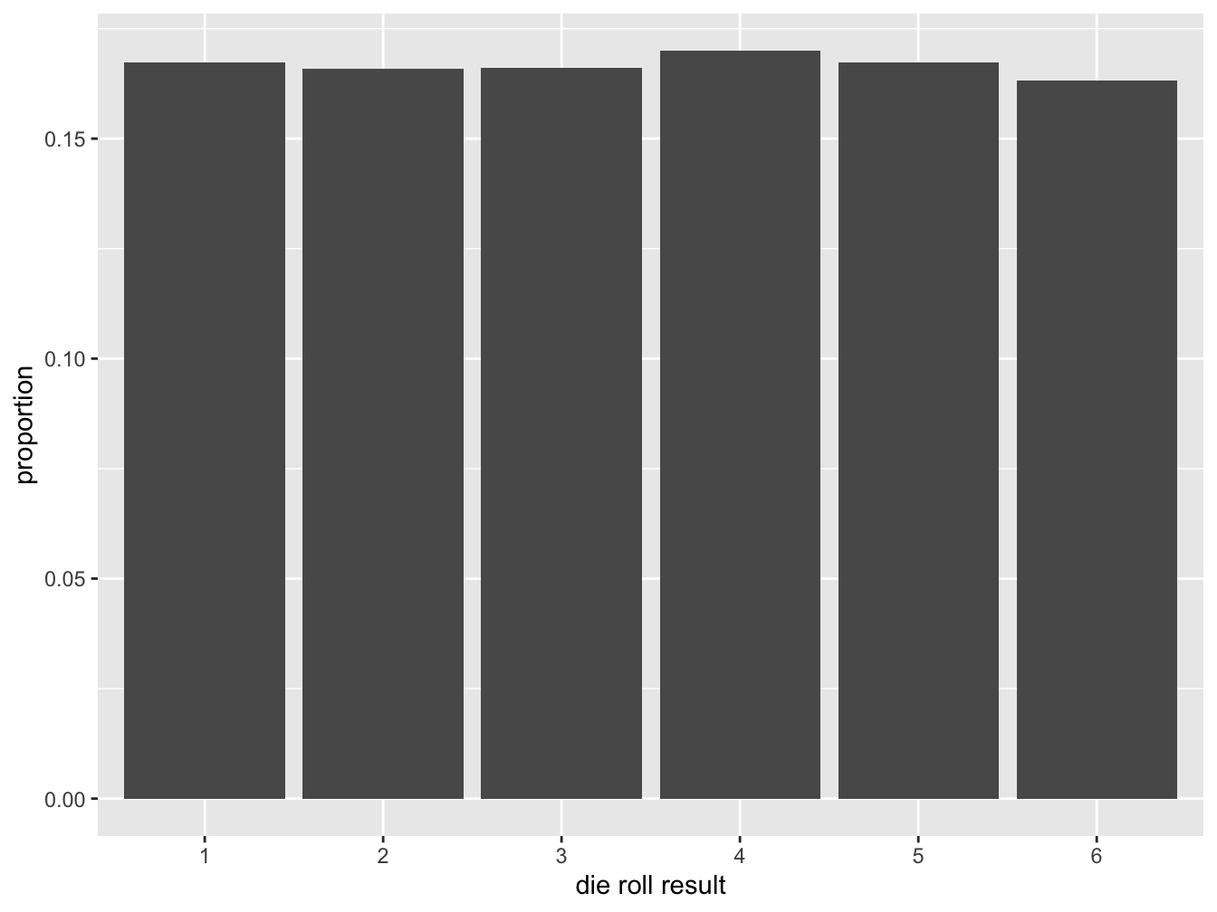
Figure 1.2: Relative Frequency Histogram for Tossing One Die
An event is any well-defined outcome of the probability experiment. For this experiment of rolling a die, one example of an event would be the outcome of rolling an even number.
We often use function notation when describing probabilities. For a well-defined event A in a probability experiment we will use P(A) to represent the probability event A occurs. We also informally use short descriptions of events combined with probability function notation as long as the context is clear. For example, when tossing a die, if it is clear from the context that we mean the event of getting a six, we might write \(P(Six) = 1/6\).
The sample space is a list of all possible outcomes of a probability experiment. One desirable property of a sample space description is that the simple events we use are equally likely, meaning all have the same probability of occurring. For example, with the experiment of tossing one die the sample space is \(\{1,2,3,4,5,6\}\).
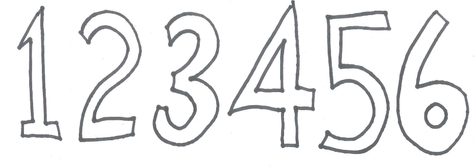
Figure 1.3: Sample Space for One Die
1.5 Simple Events
To gain some experience using sample spaces to determine probabilities consider the following simple events for the experiment of tossing one die:
- E: getting an even outcome
- S: getting a six
- L: getting a number less than three
By simply determining the ratio of successes to total members of the sample space \(\{1,2,3,4,5,6\}\), the probability of an event is found.
Getting an even can occur in three ways out of six so the probability of event E is \(3/6\). In probability notation we write \(P(E) = 3/6\).
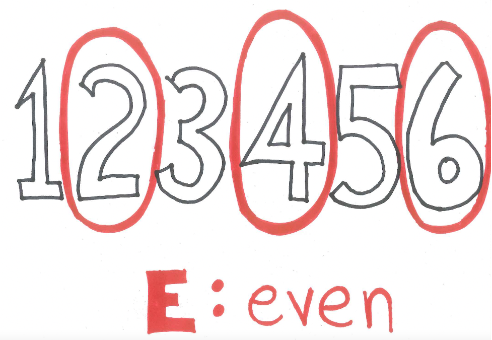
Figure 1.4: An Even Outcome on One Die
Getting a six occurs in only one of six ways so the probability of event S is \(1/6\) and expressed in probability notation as \(P(S)=1/6\).
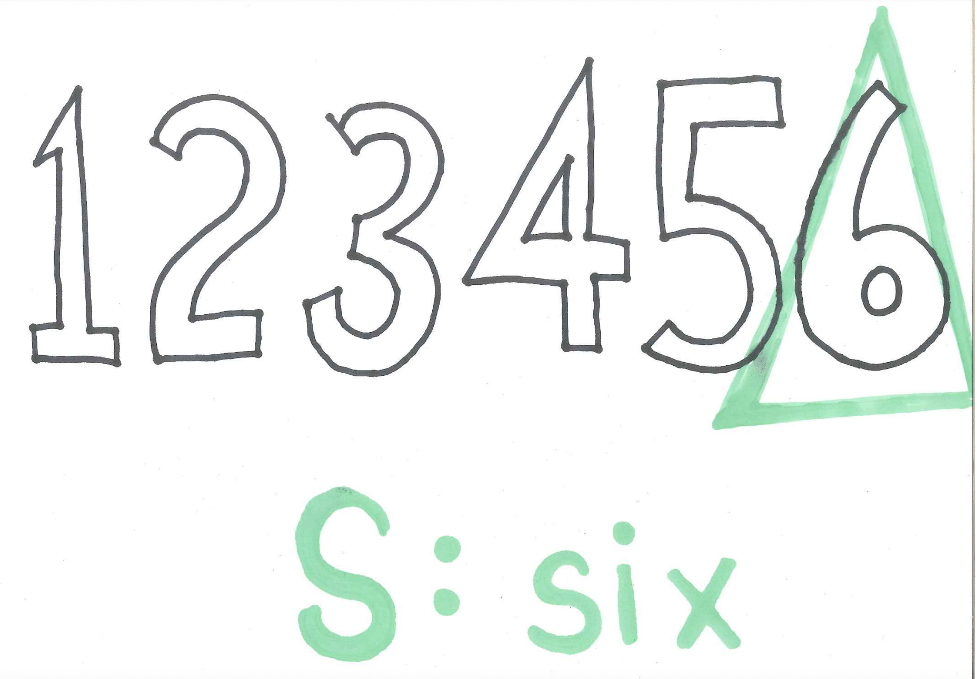
Figure 1.5: An Outcome of Six on One Die
Getting a number less than three can occur in two ways so the probability of event L is \(2/6\) and expressed in probability notation as \(P(L)=2/6\).
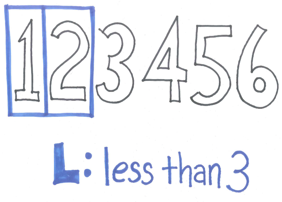
Figure 1.6: An Outcome Less Than Three on One Die
1.6 The Complement: NOT
We now consider compound events consisting of certain logical combinations of other events. We begin with the complement. The complement of an event A consists of all the outcomes that are NOT outcomes of A. We use the notation not A to represent the complement of A. (Note, some sources use \(\bar{A}\) though this can be confusing as the same symbol in other contexts represents the mean of a sample. Other sources may use yet different notation for the complement including \(E^c\) and \(\tilde E\).)
As an example, we can find the probability of the complements of the above described events for the toss of one die.
The complement of obtaining an even number is obtaining an odd number and this can happen three ways out of six so \(P(not \ E)=3/6\).
The complement of obtaining a six would be obtaining anything other than a six. This can happen five ways out of six so \(P(not \ S)=5/6\).
Be careful with inequalities. The complement of obtaining a die result less than three would be obtaining a die result greater than or equal to three. This can happen four ways out of six so \(P(not \ L)=4/6\).
1.6.1 The Complement Principle
Observe the relationship between \(P(A)\) and \(P(not \ A)\) for different events. Just as the chance of getting rain and the chance of not getting rain add to \(100\%\), we see that the probabilities of an event and its complement add to 1. This relationship between the probability of an event and its complement is called The Complement Principle which will be a very important problem-solving tool.
Theorem 1.1 (The Complement Principle) For all events A, \(P(A)+P(not \ A) = 1\).
An alternative version of the Complement Principle reads \(P(A) = 1 - P(not \ A)\).
1.7 Compound Events: AND
When we talk about the compound event A and B we mean the event where both events A and B occur. As an example, if we were considering the sample space of students in class and we were interested in the event “Female and Sophomore” only individuals who are female sophomores would qualify. Again, different texts use different notation so don’t be surprised to see on different occasions \(A \ and \ B\) as well as \(A \ \& \ B\) or even \(A \cap B\) and sometimes \(A \wedge B\). We just can’t seem to agree on one symbol. We will most often use \(A \ and \ B\) to represent the compound event of both A and B occurring.
For the experiment of tossing one die and the events defined above, we can find the probability of \(E \ and \ S\), \(E \ and \ L\), as well as \(S \ and \ L\).
The only member of the sample space that is both even and six is six itself so \(P(E \ and \ S)=1/6\).
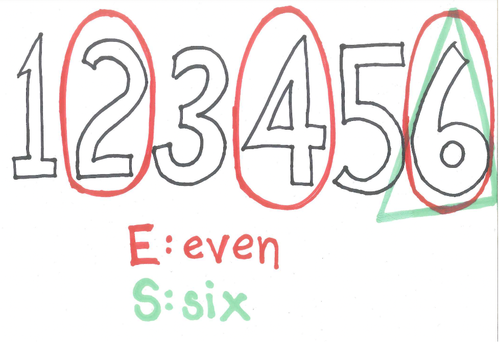
Figure 1.7: Being Both Even and a Six on One Die
The only member of the sample space that is both even and less than three is two so \(P(E \ and \ L)=1/6\).
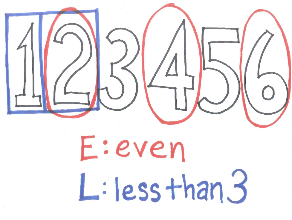
Figure 1.8: Being Both Even and Less Than Three on One Die
Examining the sample space to find elements that are both six and less than three we see there are no such creatures. Thus, \(P(S \ and \ L)=0\).
1.7.1 Mutually Exclusive Events
When two events cannot occur at the same time we say they are mutually exclusive or, equivalently, disjoint. For example, the events of selecting a Sophomore student and selecting a Junior student from our class are mutually exclusive events.
For the experiment of rolling one die and the events E, S, and L defined above, we see events S and L are mutually exclusive since one cannot roll a six and a number less than three at the same time on the same die. This is indicated in the diagram below showing there is no overlap.
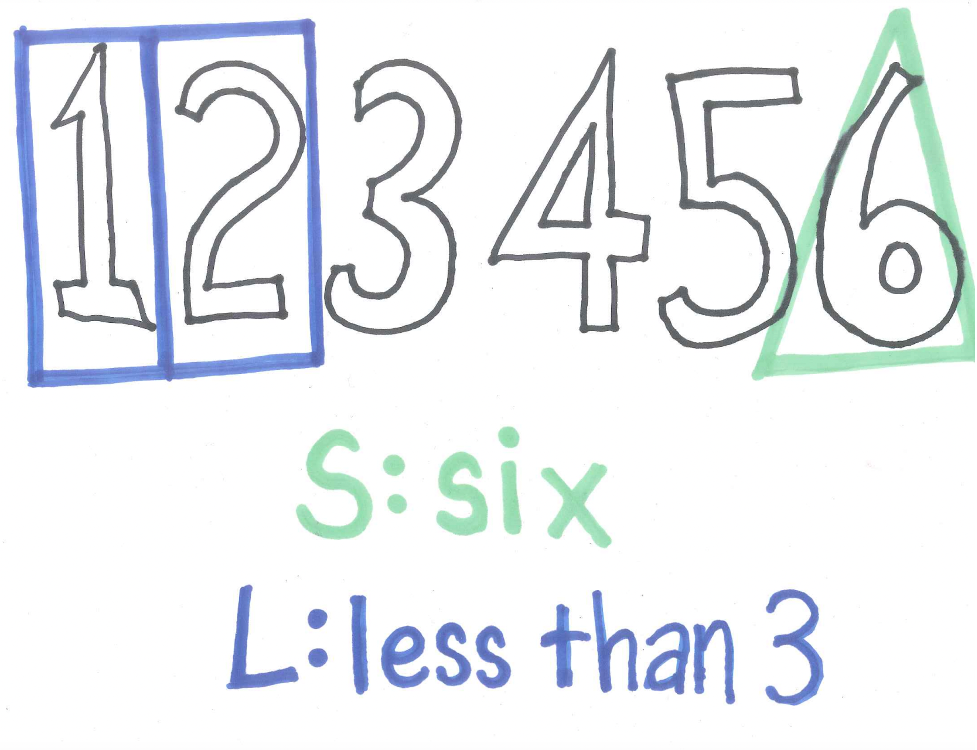
Figure 1.9: Being Both a Six and Less Than Three on One Die Cannot Occur
Here is the precise definition of mutually exclusive events:
Definition 1.1 (Mutually Exclusive) Events A and B are mutually exclusive if and only if \(P(A \ and \ B)=0\).
1.8 Compound Events: OR
We now consider the compound event E or F meaning that either event E occurred or event F occurred or both occurred. We call this an inclusive or. As an example, if we were considering the sample space of students in class and we were interested in the event of selecting a “Male or Sophomore” then this includes all individuals who are male, who are sophomore, or who are both male and sophomore.
For the experiment of rolling one die and the events defined above, we can find the probability of the event \(E \ or \ S\), \(E \ or \ L\), as well as \(S \ or \ L\).
In the image of the sample space below we see that after circling the elements that are even and marking the element that is six, a total of three elements are identified. Thus, \(P(E \ or \ S)=3/6\).
Figure 1.10: Three Outcomes are Even or a Six
In the image of the sample space below, we see that after circling the elements that are even and boxing the elements that are less than three, a total of four elements are identified. Thus, \(P(E \ or \ L)=4/6\).
Figure 1.11: Four Outcomes are Even or Less Than Three
In the image of the sample space below we see that after putting a triangle around the element six and boxing the elements that are less than three, a total of three elements are identified. Thus, \(P(S \ or \ L)=3/6\).
Figure 1.12: Three Outcomes are Less Than Three or a Six
1.8.1 Minding the Overlap
Suppose someone notices that \(P(S \ or \ L) = P(S) + P(L)\). When will a fact like this be true and when not? In examining the sample spaces above we see that events S and L are mutually exclusive. In this case, the probability of one event or the other will be the sum of the two individual probabilities.
In the other cases, we see the events are not mutually exclusive. Events E and L share the element two and events E and S share the element six. In these cases, we cannot add the individual probabilities to find the probability of one or the other because elements in the overlap will be counted twice.
In a later chapter, these insights are summarized in the Addition Principle and Special Addition Principle.
1.9 Compound Events: Conditional Probability
We consider one more way of “connecting” simple events to form a compound event. The conditional event \(X|Y\) means the event X given we know event Y occurred and we pronounce it “X given Y”. As an example, if we were considering the sample space of students in class and we were interested in the event \(Female \ | \ Sophomore\) we would mean given Sophomores only, what is the probability of being Female. Note, this is different from \(Sophomore \ | \ Female\) which is the probability you are Sophomore given you are Female.
Tossing one die with the events as described above, \(P(L \ | \ E)\) represents the probability of L given we know E occurred, that is, the probability of a number less than three given we know the number is even. Knowing it is even narrows down the sample space to three options, \(\{2,4,6\}\).
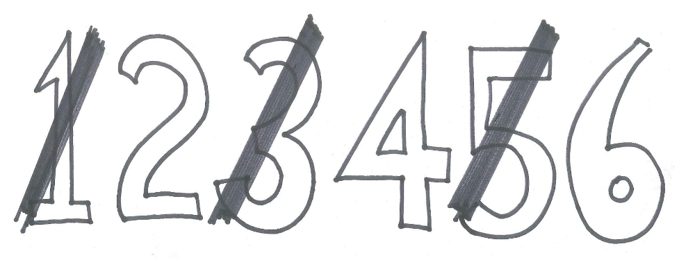
Figure 1.13: Revised Sample Space Given it is Even on One Die
Of those three options, only one of those is less than three, thus, \(P(L \ | \ E) = 1/3\).
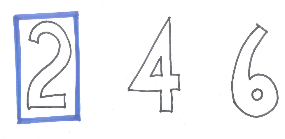
Figure 1.14: Being Less Than Three Given it is Even on One Die
Conditional probabilities are very important and a little more practice is in order. First, we note that the event \(L \ | E\) means something different than the event \(E \ | L\). To find \(P(E \ | L)\) we note that given event L occurred means the new sample space has just two elements, \(\{1,2\}\).
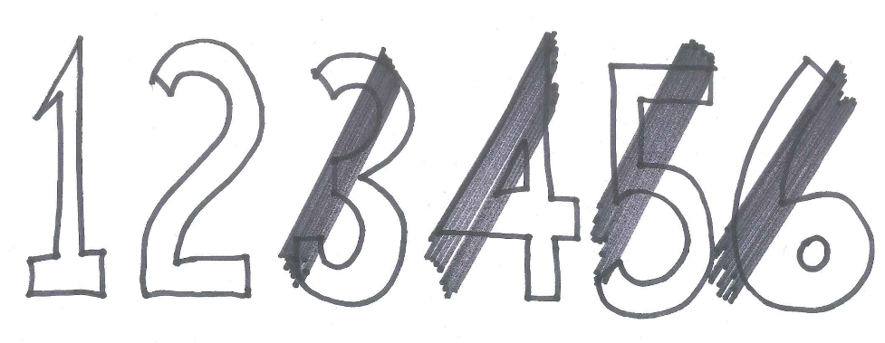
Figure 1.15: Revised Sample Space Given it is Less Than Three on One Die
And of these two options only one is even. Thus, \(P(E \ | L)=1/2\).

Figure 1.16: Being Even Given it is Less Than Three on One Die
Consider the event $ S | E$. Given that event E occurred we know the outcome is even so our new sample space has only three outcomes, \(\{2,4,6\}\). Of these, one is a six. Thus, \(P(S \ | E)=1/3\).

Figure 1.17: Being Six Given it is Even on One Die
The event \(E \ | S\) has a different meaning. Given that event S occurred we know the outcome was a six so the new sample space has only this one outcome, \(\{6\}\), and it is even. Thus, \(P(E \ | S)=1/1=1\).

Figure 1.18: Being Even Given it is a Six on One Die
To find \(P(S \ | \ L)\) we restrict our sample space to the two outcomes, \(\{1,2\}\), where L occurred and note that neither of them is six. Thus, \(P(S \ | \ L)=0/2=0\).

Figure 1.19: Being Six Given Less Than Three on One Die
In this case, \(P(L \ | \ S)\) is also 0 since if we are given event S we know that L could not have occurred. Because events L and S are mutually exclusive we see that \(P(L \ | \ S)=0\).
1.9.1 Observations about Conditional Probability
As we develop our probabilistic thinking ability, we will learn a lot about the power of conditional probability. Here are some initial observations.
First, note that, in general, for events A and B, \(P(A \ | \ B)\) means something very different from \(P(B \ | \ A)\) and, consequently, the probabilities are usually different.
Second, note in cases where the events A and B are mutually exclusive that \(P(A \ | \ B)=0\).
Third, in some cases, the conditional probability is the same as the original probability. Interestingly, in our examples above, \(P(L)\) and \(P(L \ | \ E)\) are equal. This means that event E gave us no information about the occurrence of L and we say that events E and L are independent. When knowledge that E occurred did not change the probability of L occurring and we say these two events are independent. Here is the formal definition.
Definition 1.2 (Independence) Event A and B are independent if and only if \(P(A \ | \ B)=P(A)\).
Note that if A and B are independent then not only does \(P(A \ | \ B)=P(A)\) but it is also true that \(P(B \ | \ A)=P(B)\). If two events are not independent we may say that they are dependent.
1.10 The Three Card Game Revisited
We consider the game described in the chapter scenario. Three cards – one blue on both sides, one red on both sides, and one blue on one side and red on the other - are shuffled (both interspersed and randomly turned over) and one card is randomly placed face down on the table. If the other side of the card has a different color, you win \(\$1\) while if the other side of the card has the same color you lose \(\$1\).
Here is one common faulty analysis of this situation: Once you see the color of the side that is showing this narrows down the possibilities to two - 1) the card with the same color on the other side, and 2) the card with the other color on the other side - thus, mistakenly, we might believe there is a 50/50 chance the other side has the same color.
There is a subtle error in the above thinking. While we are correct in seeing there are only two possible cards we are incorrect in thinking they are equally likely. It turns out, we are more likely to have been shown the card with same color on both sides. Thus, the error is we selected a sample space in which the outcomes are not equally likely.
In order to make sure we obtain a sample space with equally likely outcomes we might create an artificial distinction so we can tell similar events apart. Suppose we mark the two sides of the blue card as B1 and B2, the two sides of the red card as R1 and R2, and the two sides of the other card as B3 and R3. Then the sample space of which side we have been shown is \(\{B1, B2, R1, R2, B3, R3\}\) and, because the cards have been randomly shuffled and turned, each of these are equally likely.
Out of these six elements of the sample space, in four of the cases the other side of the card the same color - B1, B2, R1, R2 - and in only two cases - B3, R3 - is the other side the opposite color. Thus, the probability the other side is the same color is \(4/6=2/3\) and the probability the other side is a different color is \(2/6=1/3\). This makes sense because on two of the three cards we will always lose and only on the one card that is different on both sides will we win. Unfortunately, this means we are more likely to lose \(\$1\) than to win \(\$1\) and the game is not fair.
1.11 Exercises
1.11.1 Exercise - The Monty Hall Problem
You are shown three doors. Behind one is a car, behind the other two are goats. You are to choose one door. Hopefully you get the car. To spice it up, Let’s Make a Deal host, Monty Hall, who knows exactly what is behind each door, reveals a goat behind one of the doors that you have not chosen. Now, there remain two doors – the one you chose, and the other unopened door. Monty asks you if you want to switch doors. Should you?
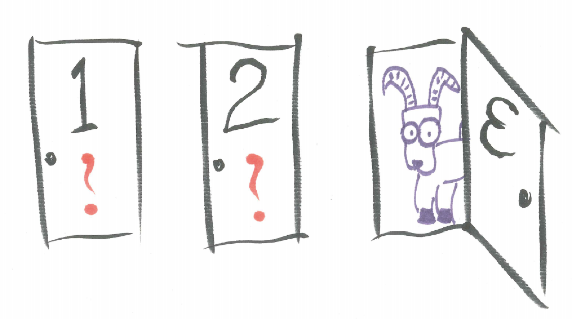
Figure 1.20: Monty Hall Problem
1.11.2 Exercise - Twelve-sided Die
Consider the different probability experiment of tossing one 12-sided Dungeons and Dragons dice. Describe the sample space and identify several events and find the probabilities of these simple events as well as at least one complement, one AND, one OR, and one conditional probability. Use probability function notation where appropriate.
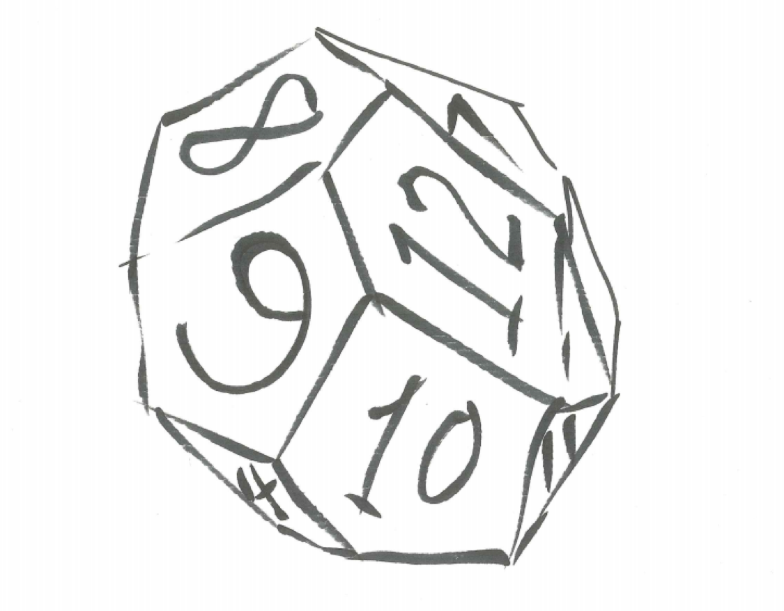
Figure 1.21: Twelve-sided Die