Chapter 23 Monte Carlo Simulation
23.1 Introduction
Simulation can give you (apparent) superpowers! It does this by leveraging experience. Rather than spend all day flipping coins (and developing rare condition of flipper’s thumbitis) we run a simulation. Financial analysts, meteorologists, astronauts, and geneticists also use simulation to test out their theories and models. In this chapter we look at random number generation in R and introduce the Monte Carlo simulation method.
23.2 Chapter Scenario - Random Darts
The standard dart board is known as the clock board and has an 18 inch diameter, that is, a 9 inch radius. Suppose that a bunch of darts are thrown and hit the board at random locations. What do you think the average distance from the center is? Would the average distance from the center be closest to 0, 1, 3, 4.5, 6, 8, or 9 inches?
23.3 About Random Number Generators
The runif(n,min=0,max=1) command with default minimum of 0 and maximum of 1 generates n random numbers between 0 and 1 from a uniform or flat distribution where the number is as likely to be any one section as in any other equally sized section. If we take a look at 1000 of these numbers and plot in a histogram we can see their distribution which should be approximately uniform or flat.
## `stat_bin()` using `bins = 30`. Pick better value with `binwidth`.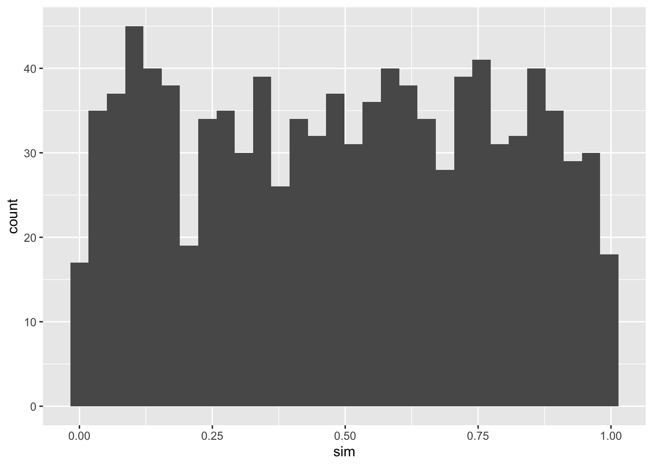
It looks a little like the New York skyline at night and not perfectly uniform because random samples vary.
The min and max parameters can be adjusted. For example, if at a particular intersection (choose your least favorite) the traffic light had a three minute long red light and we assume cars show up at the red light at random we could model the wait time of 1000 cars with runif(n=1000, min=0, max=3).
We can model random points in the plane by using runif() to select the x and y coordinates. For example, given the region in the xy-coordinate plane with x between -1 and 1 and y between -1 and 1, we can choose 1000 points at random in this region.
x <- runif(n=1000, min=-1, max=1)
y <- runif(n=1000, min=-1, max=1)
plane <- data.frame(x,y)
ggplot(data=plane, aes(x=x, y=y)) + geom_point()
We might think we see patterns but this is what random points look like.
23.4 Chapter Scenario Revisited - Random Darts
Darts are thrown at random and hit a round 18 inch diameter dart board. To estimate the average distance from the center we can generate a number of random points in a region representing the dart board, determine each point’s distance from the center, and find the average of these distances.
Let’s start by generating points in a square region of the plane with x and y both between -9 and 9.
x <- runif(n=1000, min=-9, max=9)
y <- runif(n=1000, min=-9, max=9)
plane <- data.frame(x,y)
ggplot(data=plane, aes(x=x, y=y)) + geom_point() +
  coord_fixed(ratio = 1)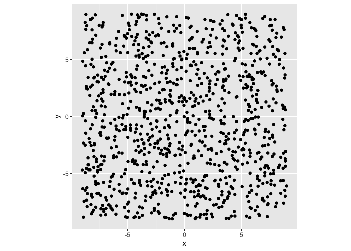
We need to select only these points that would be on a circular dartboard of radius 9. The equation of a circle of radius 9 centered at the origin is \(x^{2}+y^{2}=9^{2}\) and the interior of the circle is all points such that \(x^{2}+y^{2} < 9^{2}\) and we can select all of these rows from the dataframe plane and call it dartboard.
dartboard <- plane[plane$x^2+plane$y^2 < 81,]
ggplot(data=dartboard, aes(x=x, y=y)) + geom_point() + coord_fixed(ratio = 1)
Nice, random darts! Now we can create a new variable distance using the Pythagorean Theorem distance formula.
##            x          y distance
## 1  2.6812408  5.5383754 6.153264
## 2 -8.0089604  0.8604449 8.055049
## 3 -6.6708524 -1.8723648 6.928638
## 4 -3.4267511  0.4348523 3.454232
## 6  4.3905381 -3.8079460 5.811822
## 8  0.7586528 -3.6448880 3.723005
We can visualize these distances.
## `stat_bin()` using `bins = 30`. Pick better value with `binwidth`.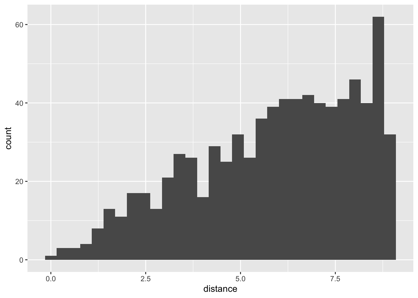
Running summary statistics.
##         min       Q1   median       Q3      max     mean       sd   n missing
##  0.03082102 4.328436 6.226172 7.764374 8.973836 5.903155 2.161193 791       0
We see the mean distance is 5.90 inches, close to 6 inches, about 2/3 of the radius. The median is a little bigger at 6.23 inches, consistent with a negatively skewed distance data.
23.5 Example - The Holey Cube
Monte Carlo Simulation is the data equivalent of throwing a large number of random darts towards a target to estimate to estimate a proportion of successes.
Here is our challenge: Imagine a cube with sides all of length four centimeters which has cylindrical holes bored out from the center of each face clear through the cube where each cylinder has a diameter of three centimeters. Check out the picture below. Since the volume of the resulting solid cannot be determined using the analytical methods of calculus, we use the Monte Carlo method to estimate the volume of the resulting solid.
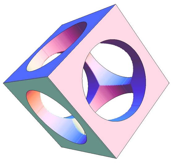
Figure 23.1: The Holey Cube
23.6 Simulating The Cube
Assume the cube has its center of mass on the origin of a three dimensional coordinate system. We simulate 10000 (x,y,z) points in the cube using the runif and matrix commands.
x <- runif(n=10000, min=-2, max=2)
y <- runif(n=10000, min=-2, max=2)
z <- runif(n=10000, min=-2, max=2)
points <- data.frame(x,y,z)
head(points)
## x y z
## 1 1.4355842 -0.2838091 -1.1370572
## 2 -0.5899566 -1.3507116 -1.8302157
## 3 -1.3021451 -1.2234585 -0.7298637
## 4 -0.6323716 1.2106794 -1.1077620
## 5 -0.6940108 -1.1407666 -1.5994467
## 6 -0.8499943 -0.6788638 0.8158404Points not in the drilled out cylinders are now identified as ones not in either of the three circles. The circle in the xy-plane is \(x^{2}+y^{2}=1\), the circle in the xz-plane is \(x^{2}+z^{2}=1\) and the circle in the yz-plane is \(y^{2}+z^{2}=1\). By replacing equality with > we identify points not in the removed circles with the and logical connective.
points$holey_cube <- points$x^2+points$y^2>1 &
                     points$x^2+points$z^2>1 &
                     points$y^2+points$z^2>1
head(points, n=10)
## x y z holey_cube
## 1 1.4355842 -0.2838091 -1.1370572 TRUE
## 2 -0.5899566 -1.3507116 -1.8302157 TRUE
## 3 -1.3021451 -1.2234585 -0.7298637 TRUE
## 4 -0.6323716 1.2106794 -1.1077620 TRUE
## 5 -0.6940108 -1.1407666 -1.5994467 TRUE
## 6 -0.8499943 -0.6788638 0.8158404 TRUE
## 7 -0.6286035 1.6807813 1.2995039 TRUE
## 8 0.5442574 -0.6559936 -0.8069817 FALSE
## 9 -0.5487874 0.6407869 1.6537750 FALSE
## 10 -0.6023055 -0.4900964 0.5878563 FALSESince points is a logical variable with \(1=TRUE\) we can sum the points variable to see how many and what proportion of the 10,000 points are left.
## [1] 5891In our simulation, 5891 of the 10000 points still remain after the holes are drilled, or 58.91 \(\%\) of the points.
## [1] 0.5891Since the original cube was of volume \(4^{3}=64\) cubic centimeters the remaining volume is 58.91 percent of 64.
## [1] 37.7024The holey cube has a volume of 37.7024 cubic centimeters.
23.7 Exercises
23.7.1 Exercise - City Grid
In 1877, Lewis Haupt, Professor of Civic Engineering at the University of Pennsylvania, laid out his ideas for urban planning including the street design below.
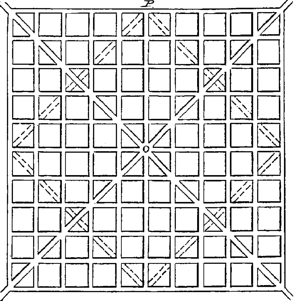
Figure 23.2: Haupt Urban Planning Model
If the city grid was one mile square mile, use the Monte Carlo method to determine the average distance from the center.
Sources: http://urbanplanning.library.cornell.edu/DOCS/haupt_77.htm http://urbanplanning.library.cornell.edu/DOCS/haupt_95.htm#hauptbio