Chapter 2 Tree Diagrams
2.1 Introduction
In this chapter, tree diagrams are introduced as important tools to analyze probability questions.
2.2 Chapter Scenario - Kitty Litter
Turns out much to our surprise the new cat was PREGNANT! Now, we have four little kittens we are not sure what to do with. They are adorable. Wonder about their sex!? I think that the most likely possibility is two female kittens and two male kittens. My partner begs to differ and thinks a 3-1 split is more likely. Can you help us out by thoroughly analyzing this situation and clearly explaining which of us is right? We have a bet and I don’t want to be the one to take out the litter box for the next year!
2.3 Example - Flipping Two Coins
Imagine a simple situation where two coins are tossed and the number of heads is observed and the outcome has some relevance for you depending on whether the result yields 0, 1, or 2 heads. Do you think each of these outcomes is equally likely? What do you think is the probability of each of these outcomes?
We use this coin-flipping scenario as a primary example not because we have inherent interest flipping coins but because this scenario is an effective model for many real-world situations such as gene inheritance.
We can review probability terminology, run a simulation, and then see how tree diagrams help us analyze this situation.
2.4 Terminology Review
We have described probability as the measure of the likelihood of an event on a scale of 0 to 1 with 0 meaning certain failure and 1 meaning certain success.
\[Probability = \frac{successes}{total}\]
Consider a coin is flipped and we examine whether it lands on heads or tails. We say it is a fair coin if heads and tails are equally likely. In this case, the probability of the coin landing on heads is \(1/2\) which can also be expressed as \(0.5\) or \(50\%\) meaning that as the experiment is repeated the proportion of heads ultimately approaches \(0.50\). Of course, sample vary so in any given number of trials the result may not be exact.
The probability experiment of flipping a coin twice and counting the number of heads leads to three possible outcomes - 0 heads, 1 head, or 2 heads but this might not be a useful sample space because these three outcomes may not be equally likely. To explore this, we could gather data by performing the experiment many times and recording the outcome but in this case a simulation might be faster and provide a larger sample much more quickly. Besides, you may not have a coin in your pocket.
2.5 Simulation
Simulation is often a helpful tool to explore probability questions like the question above regarding whether getting 0, 1, or 2 heads when flipping two coins are all equally likely. The code below simulates 10,000 trials of two coin flips keeping track of the number of heads, number of tails, and proportion of heads for each trial.
sim_2 <- do(10000)*rflip(n=2, prob=1/2)
knitr::kable(
  head(sim_2), caption = 'Table 1: Two Coin Simulation',
  booktabs = TRUE
)| n | heads | tails | prop |
|---|---|---|---|
| 2 | 0 | 2 | 0.0 |
| 2 | 0 | 2 | 0.0 |
| 2 | 1 | 1 | 0.5 |
| 2 | 2 | 0 | 1.0 |
| 2 | 1 | 1 | 0.5 |
| 2 | 2 | 0 | 1.0 |
The result is visualized in a histogram of the heads variable showing the frequency of obtaining 0, 1, and 2 heads.
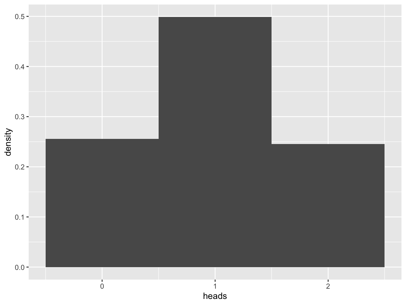
Figure 2.1: Histogram for Number of Heads When Flipping Two Coins
Examining the histogram we see that obtaining one head is more likely than the other two options and, thus, getting 0, 1, and 2 heads when flipping two coins are not equally likely outcomes. Prompted by the results of the simulation, we want to know why getting one head is more likely and tree diagrams will help us.
2.6 Tree Diagrams
The outcomes of a probability experiment can be catalogued with a tree diagram where at each node the different branches represent the different possible outcomes at each stage of the process.
Consider the tree diagram for flipping a single coin where we label each node as either H for Heads or T for tails and label the probability along each branch.
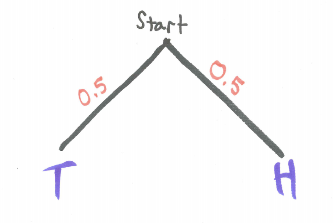
Figure 2.2: Tree Diagram for One Coin
Including the possible outcomes for a second coin results in a tree diagram with four branches.
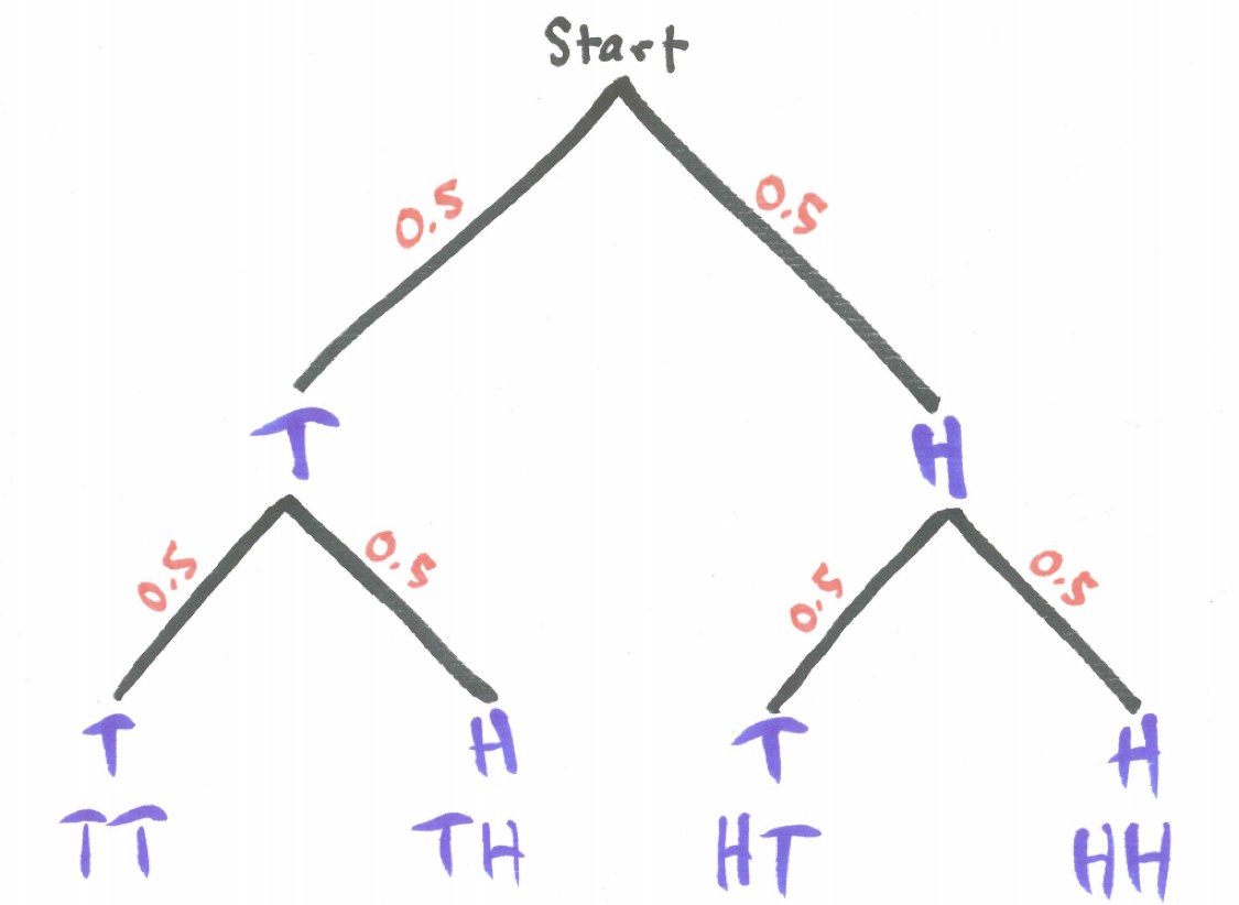
Figure 2.3: Tree Diagram for Two Coins
Each path from the top of the tree to the bottom represents one possible outcome when tossing two coins. In this experiment, there is a 50/50 chance of getting heads or tails thus all four paths are equally likely each occurring with probability \(0.5 \times 0.5 = 0.25\). If we think of the probability associated with each branch as the proportion of the time we travel down that branch then multiplying these probabilities makes perfect sense to determine the probability of traveling down sequential branches.
We can now understand why getting one head is more likely as there are two paths, HT and TH, compared to only one path generating zero heads, TT, and only one path generating two heads, HH, resulting in the following probabilities:
\[P(0\ heads) = P(TT) = (0.5)(0.5) = 0.25\] \[\small P(1\ head) = P(TH\ or\ HT) = P(TH) + P(HT) = (0.5)(0.5) + (0.5)(0.5) = 0.25 + 0.25 = 0.5\]
\[P(2\ heads) = P(HH) = (0.5)(0.5) = 0.25\]
2.7 An Example with Rats
Now consider the experiment of choosing three rats at random from a large population of rats that is 40% male and 60% female. Just as we did for coins, we can draw a tree diagram with branches representing the sex of the first, second, and third rat chosen and label the associated probabilities on each branch. Selecting the rats and identifying gender would be equivalent to having a coin that lands on one side 40% of the time and on the other 60% of the time. In the tree diagram below, we have added subscripts to identify whether we are referring to the first, second, or third rat selected.
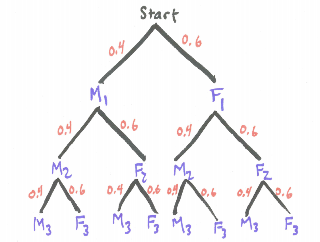
Figure 2.4: Tree Diagram for Three Rats
What is the probability of selecting 0 female rats? Note that because the population is large at each stage of the process the probability of selecting a female rat remains for all practical purposes 0.60.
\[P(0\ female\ rats) = P(M_{1}\ and\ M_{2}\ and\ M_{3}) = (0.4) \times (0.4) \times (0.4) = 0.064\]
What is the probability of selecting 1 female rat? There are actually three distinct paths through the tree where 1 female rat and 2 male rats are selected and each one has the probability \((0.6) \times (0.4)^2\) thus the probability is
\[P(1\ female\ rat) = 3 \times (0.6) (0.4)^2 = 0.288\]
2.8 Chapter Scenario Revisited - Kitty Litter
Recall our surprise - four kittens on the way! Concerning the kittens sexes, is a 2-2 or a 3-1 split is more likely? There was a bet riding on the matter. Were you able to help us? Did you use a tree diagram to visualize the sample space?
We can let F represent the event of a female kitten and M represent the event of a male kitten. We can use subscripts 1, 2, 3, and 4 to represent the first-born, second-born, and so on.
A tree diagram will show us there are 16 possible birth orderings by sex. Assuming that getting a female kitten and getting a male kitten are equally likely events, all branches in this tree are equally likely.
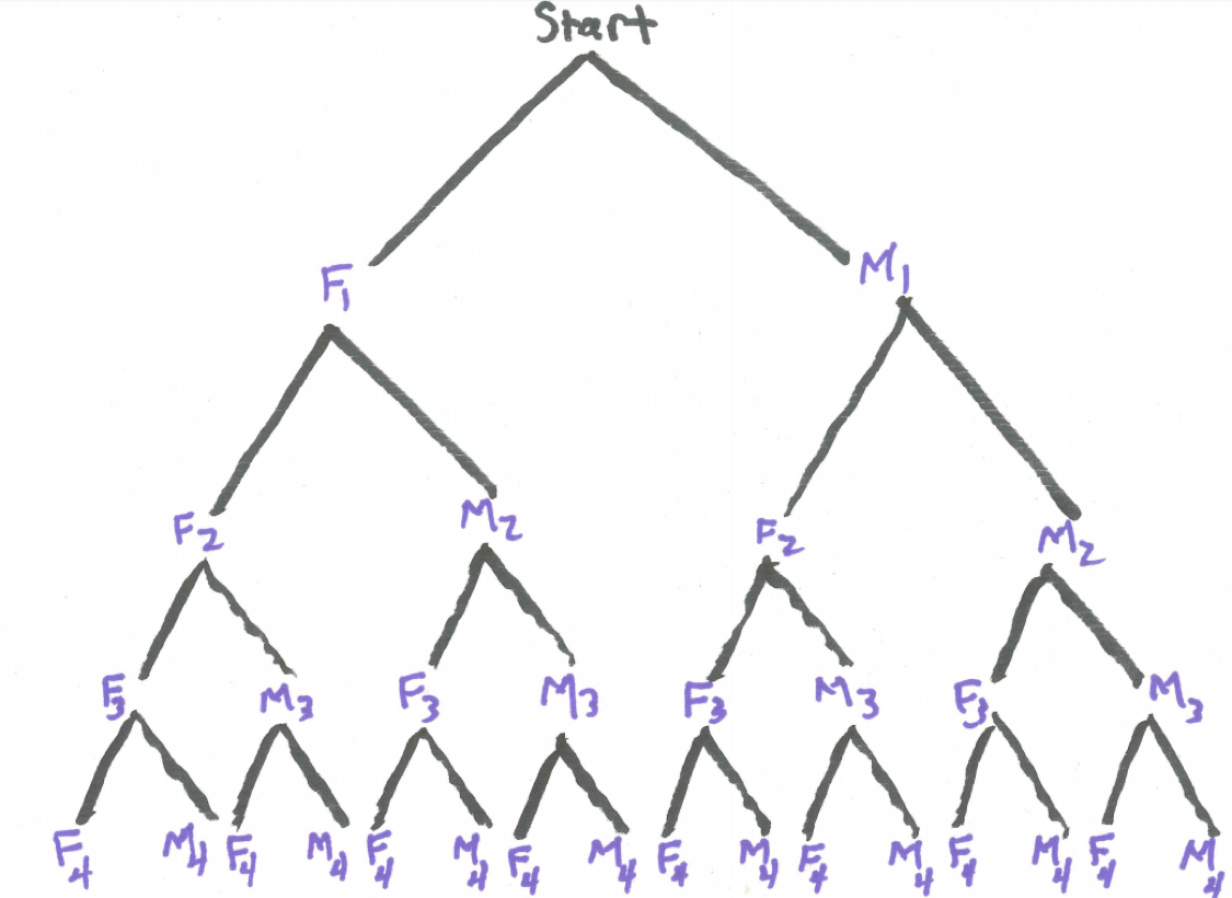
Figure 2.5: Tree Diagram for Four Kittens
Counting branches, we see there are six branches with a 2-2 sex split of two female kittens and two male kittens. Thus, the probability of a 2-2 sex split is \(6/16\).
Again counting branches, there are eight branches with a 3-1 sex split of either three females and one male or three males and one female. Thus, the probability of a 3-1 sex split is \(8/16=1/2\).
Therefore, the 3-1 split is more likely than the 2-2 split. Is it possible they can be trained to enjoy the go out of doors and not in the house?
2.9 The Urn Model
When confronted with a question of personal importance to you where probabilistic concerns are relevant to getting an accurate answer, the ability to develop a model that captures important probability details is a key problem-solving tool. By model we mean a systematic description that shares all of the important characterics of the problem, be it a physical, visual, mathematical, or computational representation (http://www.dictionary.com/browse/model).
For probability experiments two useful models are the coin-flipping model and the urn model. We have already looked briefly at a coin-flipping experiment. We will see throughout our probabilistic treatment of genetics that we will often use coin-flipping as a mental model to think about questions of genetic risk and reward. The urn model is another important way to think about probability questions.
Consider an urn with some beads in it. Imagine the urn has 20 beads 12 of which are black and 8 white and we are to draw out three of these beads at random and we want to find the probability of ending up with 0, 1, 2, or 3 black beads.
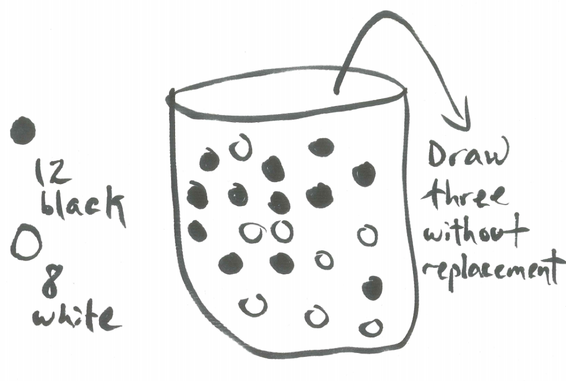
Figure 2.6: The Urn Model
First, we need to be clear up one question: is the drawing out of beads to be done with replacement or without replacement? By with replacement we mean that after each draw of one bead, it is replaced, the beads thoroughly mixed, before another bead is selected at random. By without replacement we mean that after one bead is removed, it is not replaced before the next bead is selected. Note, if we are selecting three beads at once this could be viewed as equivalent to selecting the beads one at a time without replacement.
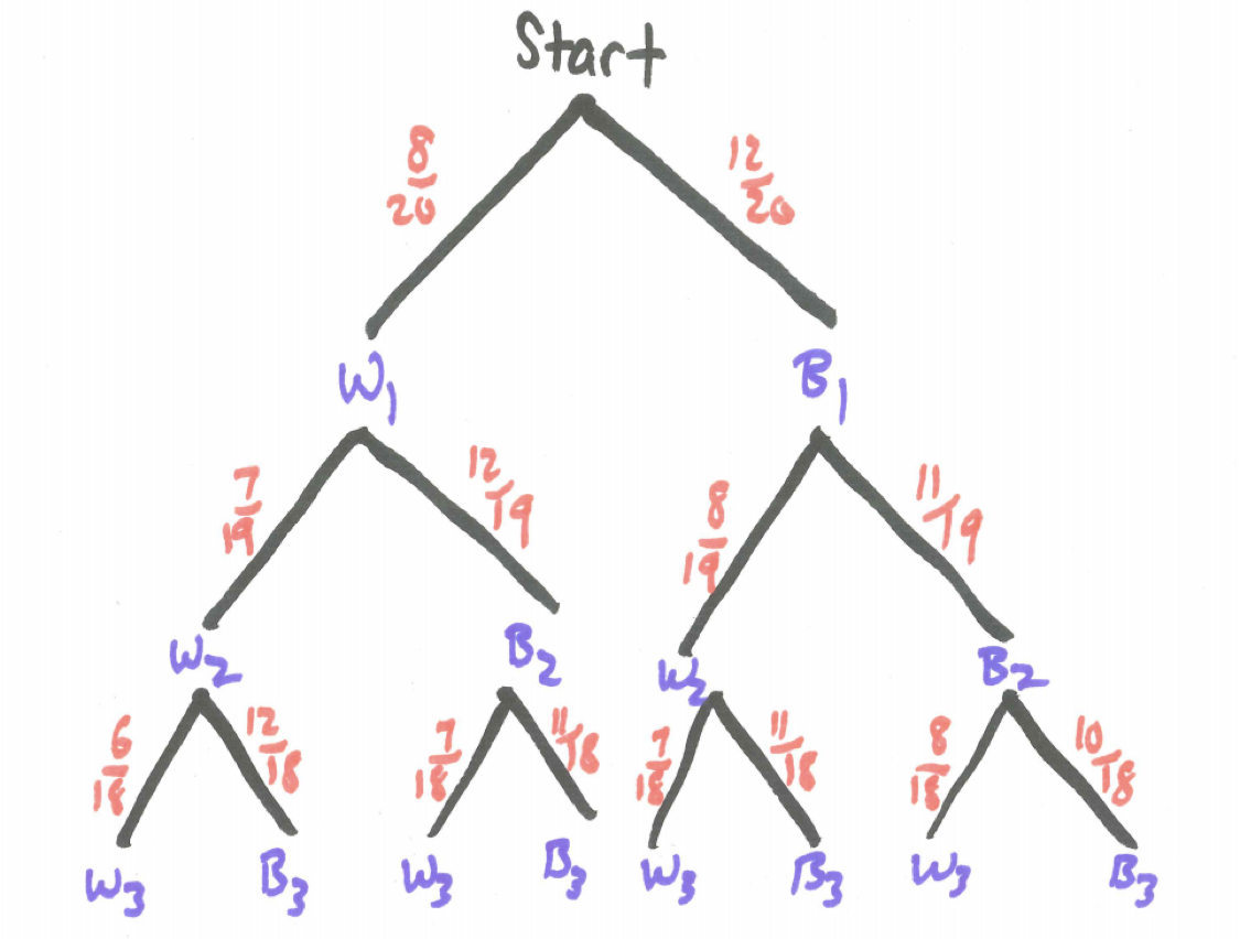
Figure 2.7: Tree Diagram for Three Beads
For this experiment with three beads drawn at random without replacement from an urn containing 12 black and 8 white beads, what is the probability of ending up with 0, 1, 2, or 3 black beads, respectively?
First, let’s tackle the probability of getting 0 black beads. From examining the tree we see
\[P(0\ blacks) = P(W_{1}\ and\ W_{2}\ and\ W_{3}) = \frac{8}{20} \times \frac{7}{19} \times \frac{6}{18}\]
Finding the probability of one black is more work. As we examine the tree we see there are three distinct paths resulting in one black. Check out their separate probabilities here.
\[P(B_{1}\ and\ W_{2}\ and\ W_{3}) = \frac{12}{20} \times \frac{8}{19} \times \frac{7}{18} = 0.098\]
\[P(W_{1}\ and\ B_{2}\ and\ W_{3}) = \frac{8}{20} \times \frac{12}{19} \times \frac{7}{18} = 0.098\]
\[P(W_{1}\ and\ W_{2}\ and\ B_{3}) = \frac{8}{20} \times \frac{7}{19} \times \frac{12}{18} = 0.098\]
In spite of the numerators being in different orders, we notice that these three separate probabilities are numerically equal. Thus, for the final probability we see
\[P(1\ black) = 3 \times \frac{12}{20} \times \frac{8}{19} \times \frac{7}{18} = 0.295\]
2.9.1 Practice
For the urn described above containing 12 black and 8 white beads with three beads drawn at random without replacement, what is the probability of obtaining two black beads? What is the probability of obtaining three black beads?
2.9.2 An Urn Model with Replacement
Consider a situation where an urn contains beads that are drawn with replacement. This means that after one bead has been randomly selected, its color is noted and it is replaced in the urn before the second one is randomly drawn and after each draw the bead is replaced. In this context, the composition of the urn remains the same and the probabilities do not change meaning that what happens when drawing one bead is independent of what happens on another draw.
An urn model where beads are drawn with replacement can represent many probability experiments. Consider the chapter scenario. An urn model representing examining the sex composition of four kittens would be an urn containing two beads, one white and one black, where the white bead represents a female kitten and a black bead represents a male kitten. From this urn, four beads would be drawn at random with replacement.
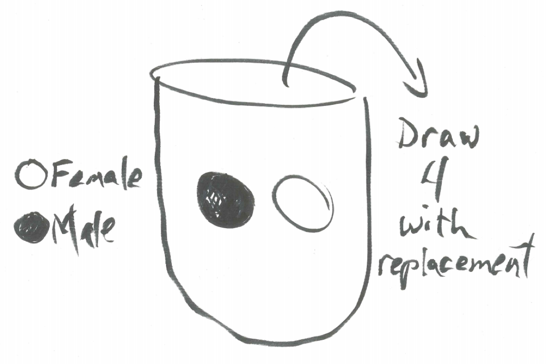
Figure 2.8: An Urn Model for Four Kittens
2.10 Exercises
2.10.1 Exercise - Three Coins in the Fountain
A penny, a nickel, and a dime are all flipped at the same time. Draw an appropriate tree diagram with associated probabilities labeled on each branch and find the probabilities of the following events: obtaining no heads, obtaining exactly one head, exactly two heads, and exactly three heads.
2.10.2 Exercise - More Coins
Draw a tree diagram for the probability experiment of flipping four coins. Label each node as either H for Heads or T for tails and label the probability along each branch. Find the probability of obtaining no heads and the probability of obtaining at least one head and describe the relationship between these two probabilities.
2.10.3 Exercise - Class Committee
Consider the experiment of selecting a committee of three individuals from a class of 20 of which 8 are male and 12 are female. Draw a tree diagram with associated probabilities for the sex of the first, second, and third person chosen for the committee and find the probabilities the committee consists of 0 females, 1 female, 2 females, and 3 females, respectively.