Chapter 19 The Poisson Distribution
19.1 Introduction
We have learned about important discrete random variables such as the binomial and about important continuous random variables such as the normal. In this chapter we add to our repertoire some other useful distributions including the geometric, negative binomial, and poisson discrete random variables and the uniform and exponential continuous random variables.
19.2 The Poisson Random Variable
19.2.1 The Poisson Distribution
The Poisson distribution is often used to model real-world phenomena related to the number of certain events that occur over a specified period of time such as the number of math errors made in a typical math class, the number of text messages received during class, or even the chance of an earthquake occurring sometime this semester.
A discrete random variable X is said to have a Poisson distribution with parameter \(\lambda>0\), if, for \(k=0,1,2,...\), is denoted as \(X \sim POI(\lambda)\) with the probability mass function of X given by
\[P(X=k)=\frac{\lambda^{k}*e^{-\lambda}}{k!}\] This formula would determine the probability of \(k\) events occurring. The expected value for a Poisson random variable with parameter \(\lambda\) is \(E(X)=\lambda\), the variance is also \(Var(X)=\lambda\), and the standard deviation is \(SD(X)=\sqrt{\lambda}\).
19.2.2 The Poisson Random Variable in R
Assume we have a Poisson random variable with parameter \(\lambda\). We often determine \(\lambda\) by finding the sample mean from data since the expectation of a Poisson is \(\lambda\).
To find the individual probability of x occurrences, \(P(X=x)\), use dpois(x, lambda).
To find the cumulative probability of less than or equal to x successes, \(P(X \leq x)\), use ppois(q, lambda, lower.tail = TRUE).
To visualize the cumulative probability \(P(X \leq x)\) use pdist(dist="pois", lambda, q=x).
To find the inverse probability, that is the value of x such that \(P(X \leq x) = p\) use qpois(p, lambda, lower.tail = TRUE).
To generate a random sample of size n from a poisson random variable use rpois(n, lambda).
19.2.3 Modeling Number of Earthquakes with the Poisson
Consider how the Poisson can be used to model different phenomena. One key is that the parameter \(\lambda\) equals the expected value. Thus, if you know the expected value you can use this value for \(\lambda\) to find probabilities. Here we apply this technique to examine earthquake frequency along the Wasatch Front. The earthquake frequency table below is from the University of Utah Seismic Station’s website - http://www.seis.utah.edu/edservices/EES/WsatchFrontClock.shtml.
Suppose that we make the simplifying assumption that the number of earthquakes of a given magnitude that occur in a given time period is a Poisson distribution and that the estimate of the recurrence interval can be used to determine the parameter .
Suppose that we are interested in the occurrence of earthquakes of magnitude greater than 3.0 during a two-semester period of 8 months. Since the estimate of the recurrence interval is 4 months we would expect approximately two earthquakes in eight months thus we would model the number of earthquakes, X, as a Poisson with parameter \(\lambda=2\), \(X \sim POI(2)\).
To find the probability of 0 earthquakes in a two-semester period:
## [1] 0.1353353To find the probability of 1 earthquake in a two-semester period:
## [1] 0.2706706For cumulative probabilities of 2 or fewer earthquakes in a two-semester period:
## [1] 0.6766764Using the complement principle we can find the probability of more than 2 earthquakes in a two-semester period:
## [1] 0.3233236The ‘mosaic’ package in R creates fantastic visualizations of probability distributions. Examine the code below showing the probability of two or fewer earthquakes.
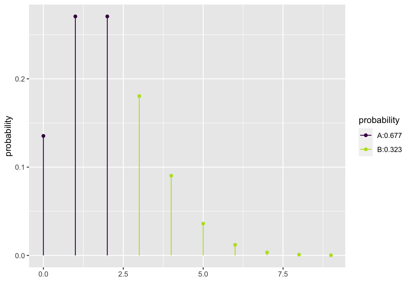
## [1] 0.6766764Thus, there is a 67.6676416 percent chance of two or fewer earthquakes in a two-semester period.
To find the 90th percentile:
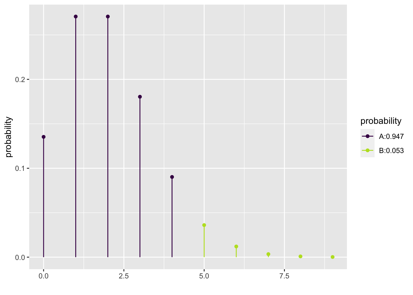
## [1] 4Thus, we can say that according to our model, there is a 90% chance of 4 or fewer earthquakes in a given two-semester period.
19.3 Exercises
19.3.1 Exercise - Counting Earthquakes
Earthquakes of magnitude greater than 3.0 along the Wasatch front occur on average every four months. Considering a two-semester period of 8 months we expect approximately two earthquakes and can model the number of earthquakes as a poisson distribution with parameter \(\lambda=2\). (a) Determine the probability of three or fewer earthquakes of magnitude greater than 3.0 in the next 8 months and llustrate this probability with a plot of the probability distribution. (b) Find the 75th percentile for the number of earthquakes of magnitude greater than 3.0 in the next 8 months and illustrate the 75th percentile with a plot of the probability distribution. (c) If we were to explore the number of earthquakes of magnitude greater than 3.0 in the next two-year period instead of the next 8 months explain what value for \(\lambda\) would be appropriate in a Poisson model.
19.3.2 Exercise - Growth Mindset and Math Errors
Psychologist Carol Dweck, in her book Mindset: The New Psychology of Success, advocated that students focus on the learning process to develop their intelligence rather than to think intelligence is fixed. In math this might mean we need to embrace making mistakes as mistakes provide the main context for exploring effective and ineffective approaches to a problem. Suppose that in an active and engaged college math class, an average of 8 math mistakes are made on the whiteboard per class session. Use a Poisson model to find the following. (a) What is the probability that in an active and engaged math class there will be 0 math mistakes made on the whiteboard in a class session? (b) Is it more likely that there will be fewer than 8 or more than 8 math mistakes made on the whiteboard in a class session? (c) One particularly productive session had 10 great mistakes from which to learn. What is the probability of 10 or more mistakes on the whiteboard in a class session?