Chapter 22 The Exponential Distribution
22.1 Introduction
We have learned about important discrete random variables such as the binomial and about important continuous random variables such as the normal. In this chapter we add to our repertoire some other useful distributions including the geometric, negative binomial, and poisson discrete random variables and the uniform and exponential continuous random variables.
22.2 The Exponential Distribution
Recall, the Poisson distribution is models the number of events that occur over a specified period of time. A related variable of interest is the time we need to wait for the next event. In a real-world situation, if the number of events in a certain period of time - be it math errors in class, earthquakes in a school year, etc. - then the time until the next occurrence can be modeled with the continuous random variable called the exponential distribution.
22.2.1 The Exponential Probability Density Function
If the average rate of an event is \(\lambda\) occurrences per period of time then wait time until the next occurrence can be modeled with an exponential random variable \(T \sim (\lambda)\) with probability density function
\[f(t)=\lambda \cdot c^{\lambda \cdot t}\]
for \(t > 0\).
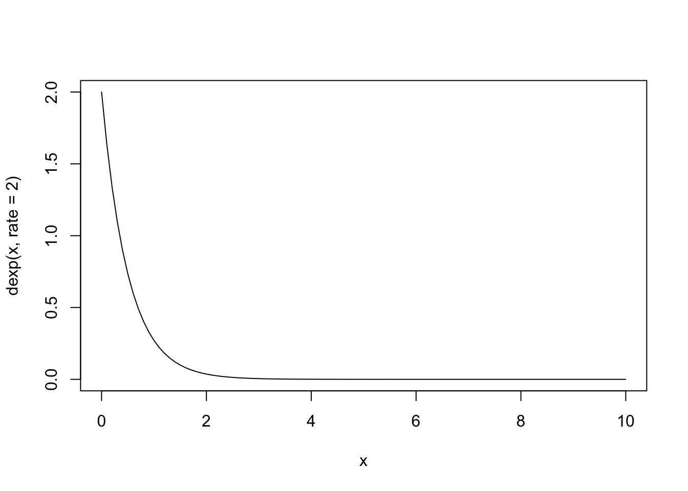
Using base graphics, here is the probability density function for an exponential random variable with \(\lambda=2\).
The expected value of an exponential random variable is \(1/\lambda\) and the variance is \(2/\lambda^{2}\), and standard deviation \(\sqrt{2/\lambda^{2}}\).
The exponential random variable can be shown to be memoryless, meaning that if a certain amount of time has passed without an occurrence this doesn’t change the expected amount of time we still need to wait.
22.2.2 The Exponential Random Variable in R
Given exponential random variable T with parameter \(\lambda\)
To find the probability of T being less than q, \(P(T < q)\), use pexp(q, rate=lambda, lower.tail=TRUE).
To find the probability of X being greater than q, \(P(X > q)\), use pexp(q, rate=lambda, lower.tail = FALSE) or 1-pexp(q, rate=lambda, lower.tail = TRUE).
To find the inverse probability, that is the value of x such that \(P(T \leq x) = p\) use qexp(p, rate=lambda, lower.tail = TRUE).
To generate a random sample of size n from a uniform random variable use rexp(n, rate=lambda).
22.2.3 Example - Soccer Wait Times
The average number of soccer goals per game in the 2014 World Cup in Brazil was 2.7 meaning the goal rate was \(2.7/90=0.03\) goals per minute. To model the time in minutes until the next goal occurs in a soccer match we can use the exponential random variable T with \(\lambda=0.03\).
The expected value or average time until the next goal is \(1/\lambda=1/0.03=33.33\) minutes.
What is the chance there will be a goal in the next 15 minutes? We want to find \(P(T < 15)\).
## [1] 0.3623718According to our model, there is a 36.2371848 \(\%\) chance of a goal in the next 15 minutes.
What are the chances there will be no goal in the next game is \(P(T > 90)\)?
## [1] 0.06720551Thus, the chance of no goal for the entire game is 0.0672055, a small probability but not that unusual.
22.2.4 Example - The Computer Help Desk
According to the latest stats, Westminster’s computer help desk receives about 20 calls per 8 hour shift for a rate of \(20/8=2.5\) calls per hour. The time T in hours until the next support call can be modeled with an exponential function with parameter \(\lambda=2.5\).
The average time until the next call is \(1/2.5=0.4\) hours or 24 minutes.
What is the probability the next call will occur sometime between 30 and 60 minutes from now. To find this probability, we need to find \(P(T < 60)\) and subtract off the unwanted region, \(P(T < 30)\).
## [1] 0The probability of a wait of between 30 and 60 minutes is 0. Do you think I have time to run down to 7-11?
22.3 Exercises
22.3.1 Exercise - Waiting on that Earthquake
Earthquakes of magnitude greater than 3.0 along the Wasatch front occur on average every four months. Considering a two-semester period of 8 months we expect approximately two earthquakes. While we can model the number of earthquakes per school year as a poisson distribution with parameter \(\lambda=2\), this might be an unusual time period to use to model the waiting time until the next one. If we used months as our unit of time, what value of the parameter \(\lambda\) would we use to model the time until the next earthquake of magnitude greater than 3.0? What would be the probability we would wait three or more months for the next earthquake of magnitude greater than 3.0?
22.3.2 Exercise - NHL Hockey Goals
During the 2017-2018 season, the home team scored on average 2.97 goals. Hockey games consist of three 20 minute periods so each game is 60 minutes. Model the time until the next goal with an exponential random variable. Find the probability that in one period, 20 minutes, there will not be a goal. Find the probability that the next goal will occur between 10 and 20 minutes from now.
Source: hockey-reference.com