Chapter 9 Measures of Variation
9.1 Introduction
When examining data key features we look for are the shape, center, spread, and unusual values. Similarly, when examining a probability distribution we can see the shape and unusual values by visualizing the probability histogram and we can determine the expected value to shed light on the center of the distribution. But these tell us nothing about one of the most important aspects of a probability distribution to understand - the spread - that is, how the outcomes vary. We use two main measures for variability - variance and standard deviation. The main idea of the variance is that it is the average squared distance from the mean. The standard deviation is the square root of the variance.
9.2 Chapter Scenario - Roulette Fun Bus
As described before, to play roulette you place a bet and spin the wheel. If the wheel matches your bet you win; if not, you lose. Remember that a roulette wheel contains slots numbered 1 through 36, half of them red, half black and green 0 and 00 slots.
Different bets have different payoff ratios. Previously, we compared the even money bet paying off at 1:1 with a single number bet paying off at 35:1 and discovered the house advantage is identical for these two bets, \(5.26\%\), in spite of the payoff odds being so different.
Imagine two giant Fun Buses headed to Wendover each with 100 people. One is the bus and the other is the bus.
On one bus (call it the conservative party bus) each person will spend the evening making 360 \(\$10\) even money bets (red, black, even, odd, high, or low).
Now, consider another bus (call it the party bus) where each person makes 360 bets of \(\$10\) each on a single number, the lucky number of their choice.
Our goal is to compare the bus ride home for these two groups. At the end of the evening, and all evenings must end, how do you expect results on the bus to compare with results on the bus in terms of shape, center, spread and unsual values? Do you expect the same distribution? Do you expect the same average winnings/losings? Do you expect the same proportion of winners? Which bus would have more big winners? Which bus would have more big losers?
9.3 Measuring Variability with Variance and Standard Deviation
To measure the spread of a random variable, we need a reference point. We use the expected value, this key measure of the center of a distribution, as our reference point. We would like to see how far from the center the values of the random variable are likely to be. For technical reasons, we find the expected value of the square of the difference between random variable X and its mean. This is called the variance. The square root of the variance is called the standard deviation and have the virtue of being in the same units as the original random variable.
9.4 Example - Roulette Even Money Bet
Suppose that \(\$10\) is bet in Roulette on red. Adapting our previous analysis we can find the expected value.
\[E[X] = \sum_{x} x \cdot P(x)=+10 \cdot \frac{18}{38}-10 \cdot \frac{20}{38}=-\frac{20}{38}=-0.526\]
To use the short-cut formula for the variance we can first find $E[X^{2}].
\[E[X^{2}]=\sum_{x} x^{2} \cdot P(x)=10^{2} \cdot \frac{18}{38}+(-10)^{2} \cdot \frac{20}{38}=\frac{3800}{38}=100\]
The variance is thus
\[Var(X)=E[X^{2}] - (E[X])^{2}=100 - (-0.526)^{2}=99.72\]
The standard deviation is the square root of the variance.
\[SD(X)=\sqrt{Var(X)}=\sqrt{99.72}=\] 9.9859902
These values can be computed in R by first inputing the probability distribution.
## [1] -0.5263158## [1] 99.72299## [1] 9.986149.5 Example - Roulette Single Number Bet
We can similarly analyze a \(\$10\) is bet in Roulette on a single number. Adapting our previous analysis we can find the expected value.
\[E[X] = \sum_{x} x \cdot P(x)=+350 \cdot \frac{1}{38}-10 \cdot \frac{37}{38}=-\frac{20}{38}=-0.526\]
To use the short-cut formula for the variance we can first find $E[X^{2}].
\[E[X^{2}]=\sum_{x} x^{2} \cdot P(x)=350^{2} \cdot \frac{1}{38}+(-10)^{2} \cdot \frac{37}{38}=\frac{3800}{38}=3226.316\]
The variance is thus
\[Var(X)=E[X^{2}] - (E[X])^{2}=3226.316 - (-0.526)^{2}=3226.039\]
The standard deviation is the square root of the variance.
\[SD(X)=\sqrt{Var(X)}=\sqrt{3226.039}=\] 56.7982306.
Using R:
## [1] -0.5263158## [1] 3320.776## [1] 57.626179.6 Example - Deal or No Deal
Earlier we examined selecting a suitcase from the 26 Deal or No Deal suitcases and discovered the expected value is \(\$131477.50\) while the theoretical median is \(\$875\). Knowing these facts might impact how much you would be willing to pay to play the game but they are not the whole story. Suitcases amounts range from 1 cent to 1,000,000 dollars. Variance and standard deviation help us quantify how variable the outcomes are.
We duplicate below the suitcase amounts and the probability vector along with calculating the expected value.
suitcases <- c(0.01, 1, 5, 10, 25, 50, 75, 100, 200, 300, 400,
       500, 750, 1000, 5000, 10000, 25000, 50000, 75000,
       100000, 200000, 300000, 400000, 500000, 750000, 1000000)
probs <- rep(1/26, 26)
deal_expectation <- sum(suitcases*probs)
deal_expectation
## [1] 131477.5Given the suitcase amounts suitcases and the mean deal_expectation and the probabilities probs we can easily compute the variance and standard deviation.
## [1] 64305084524## [1] 253584.5The standard deviation is large, approximately a quarter of a million, a reflection of the large range of possible winnings. We need to look at all of the pieces including the simulation and the theoretical analysis to better understand the situation. Suitcase amounts range from \(\$0.01\) to \(\$1,000,000\) with a mean of \(\$131,477.50\), a median of \(\$875\) and a standard deviation of \(\$253,584.50\). The mean is large but so is the standard deviation. We would need to take this into account when deciding how much we would be willing to pay for the privilege of choosing a suitcase.
9.7 Chapter Scenario Revisited - Roulette Fun Bus
Recall, we are imagining two giant Fun Buses headed to Wendover each with 100 people. On the conservative party bus, each person will spend the evening making 360 \(\$10\) even money bets. On the party bus, each person will spend the evening making 360 bets of \(\$10\) each on a single number, the lucky number of their choice. We have seen that the even money bets and the single number bets both have exactly the same house advantage, \(5.26\%\).
Our goal is to compare the two buses at the end of the evening. Will they have the same proportion of winners? Where will the big winners be? Where will the big losers be? Which bus would you rather ride home on?
9.7.1 Simulating the Bus
The code below simulates 100 people each making 360 bets of 10 dollars each on an even money bet like Red and computes the sum for each person.
red_bus <- do(100)*sum(sample(c(-10,10), size=360, prob=c(20/38,18/38), replace=TRUE))
head(red_bus)
## sum
## 1 140
## 2 -300
## 3 -400
## 4 -300
## 5 -120
## 6 -320Running favstats() on the sum variable we can see on average how much each person lost.
##   min   Q1 median  Q3 max   mean       sd   n missing
##  -660 -340   -220 -80 180 -207.2 181.8984 100       0
Examine the histogram of winnings/losings for the 100 people on the fun bus.
## `stat_bin()` using `bins = 30`. Pick better value with `binwidth`.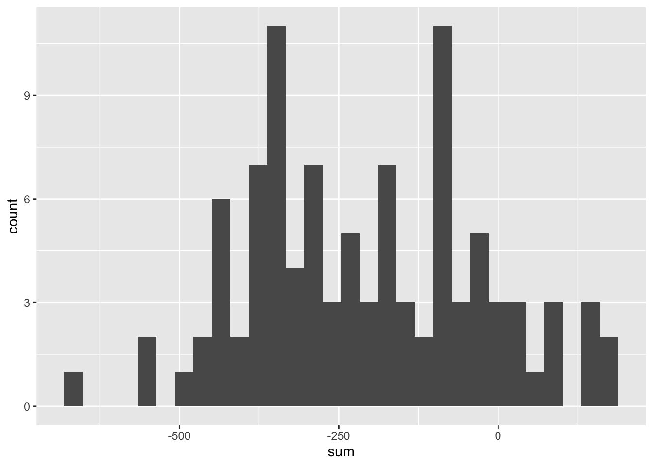
We can find the proportion of winners as follows:
## prop_TRUE
##      0.12
Summing up, we see that the average winnings on the night for these 100 people on the bus each spending the evening making 360 ten dollar even money bets on roulette was -207.2 dollars and that overall, 12% of the bus riders came out winners.
9.7.2 Simulating the Bus
Now consider the party bus where each person makes 360 bets of \(\$10\) each on a single number, the lucky number of their choice. The bus is where the real fun happens.
Adapting the code above by changing the payoffs and probabilities, we simulate 100 people each making 360 bets of 10 dollars each on an even money bet like Red and compute the sum for each person.
blue_bus <- do(100)*sum(sample(c(-10,350), size=360, prob=c(37/38,1/38), replace=TRUE))
head(blue_bus)
## sum
## 1 2160
## 2 0
## 3 360
## 4 -720
## 5 -720
## 6 -1440Running favstats() on the sum variable we can see on average how much each person lost.
##    min   Q1 median  Q3  max   mean       sd   n missing
##  -2160 -720   -180 360 2160 -169.2 983.5143 100       0
Examine the histogram of winnings/losings for the 100 people on the fun bus.
## `stat_bin()` using `bins = 30`. Pick better value with `binwidth`.
We can find the proportion of winners as follows:
## prop_TRUE
##      0.38
Summing up, we see that the average winnings on the night for these 100 people on the bus each spending the evening making 360 ten dollar single nubmer bets on roulette was -169.2 dollars and that overall, 38% of the bus riders came out winners.
9.7.3 Comparing the and Buses
We want to compare the results of two buses in terms of shape, center, spread, and unusual values.
Both distributions were somewhat mound-shaped. The centers as measured by the means were different but we would expect in both cases the average loss to be \(360 \cdot 0.526\) = 189.36. The bus lost a little more than this on average and the bus lost a little less than this on average but samples do vary.
The most significant difference between the two buses is revealed when we examine the standard deviations. The bus had a standard deviation of 181.8984065 and the bus had a standard deviation of 983.5142925 which is more than five times larger. That means that outcomes on the bus were much more variable.
When we place these simulated result in a side-by-side boxplot the difference in spread stands out.
combined_data <- data.frame(red=red_bus$sum, blue=blue_bus$sum)
double_decker <- stack(combined_data)
colnames(double_decker) <- c("winnings", "bus")
ggplot(double_decker, aes(x=bus,y=winnings, fill=bus))+geom_boxplot()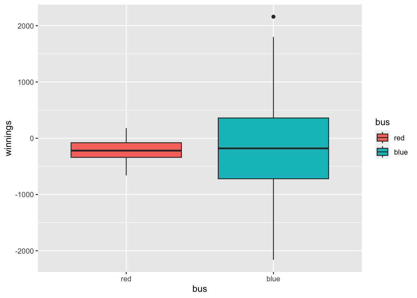
We see there were more large winners and more large losers on the bus. There was no such large winners or losers on the bus. Variation matters. Which bus would you rather be on?