Chapter 3 Multiple Events
3.1 Introduction
After being introduced to the basic terminology of probability, we want to see how probability works in more complex situations. In this chapter we tackle dealing with multiple events and using the Fundamental Counting Principle.
3.2 Chapter Scenario - The Game of Diff
Suppose the casino has hired you as a consultant to create a simple but appealing dice game. It is proposed that the player pays a certain fee and then rolls two dice. The difference between the dice is tabulated and the player receives that amount in dollars. The casino wants to know how much to charge for this game. Your job as consultant is to determine an appropriate price which, while appealing to the player, will also generate a consistent profit for the casino. To decide, first estimate what you think the average winnings for this game would be and, second, what price you think would appeal to the player but also generate a consistent profit for the casino.
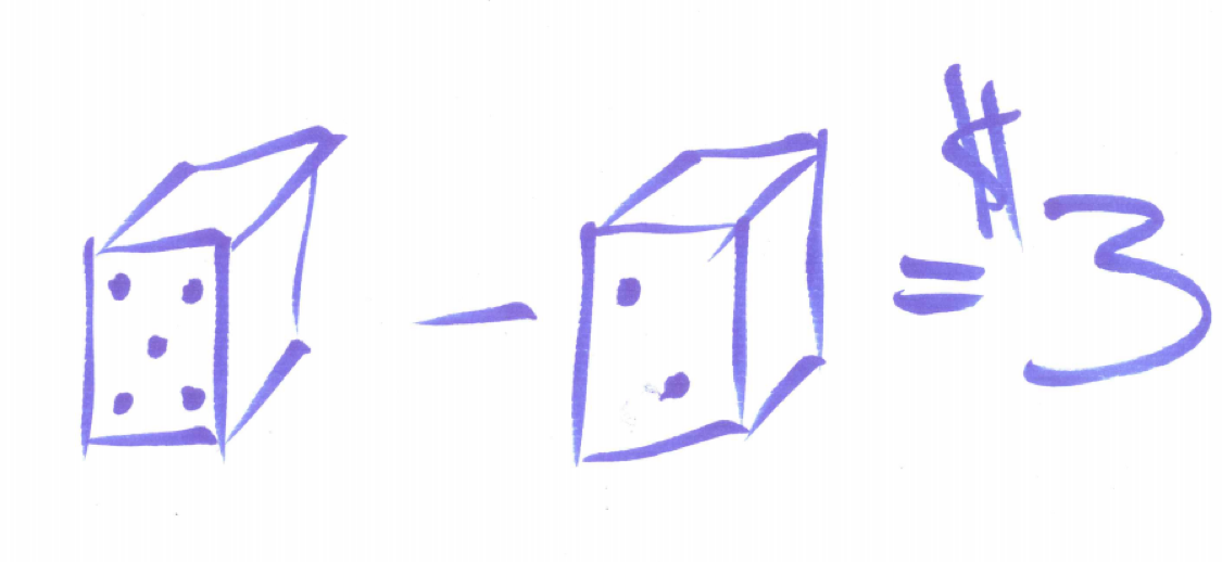
Figure 3.1: Game of Diff Example
After estimating the average winnings, play the game ten times with a partner documenting the actual difference. Based on this preliminary data does it look like you made a reasonable choice for price? Why or why not?
3.3 Example - Pair of Dice
After working with the toss of one die in the previous chapter, we examine the outcomes when tossing two dice to explore how to handle multiple events.
Earlier you examined the experiment of tossing one die. The sample space for this experiment is the set of equally likely outcomes S={1,2,3,4,5,6} and the probability of different simple and compound events can be found using this sample space.
When examining two dice, one might naively consider all the different outcomes one could get when summing the dice and proceed with a possible sample space of S = {2,3,4,5,6,7,8,9,10,11,12}. You might suspect this is not a useful sample space based on experience. It seems like getting a sum of 2 or 12 is unusual but getting a sum of 7 occurs more frequently.
The simulation below generates 10,000 tosses of two dice and their sum and helps us see that these sums are not equally likely and thus not a great sample space to work with.
die1 <- sample(x=1:6, size=10000, replace = TRUE)
die2 <- sample(x=1:6, size=10000, replace = TRUE)
sum <- die1 + die2
sim_two_dice <- data.frame(die1, die2, sum)
knitr::kable(
  table(sum), caption = 'Tossing Two Dice Simulation',
  booktabs = TRUE
)| sum | Freq |
|---|---|
| 2 | 277 |
| 3 | 565 |
| 4 | 789 |
| 5 | 1075 |
| 6 | 1386 |
| 7 | 1698 |
| 8 | 1442 |
| 9 | 1143 |
| 10 | 812 |
| 11 | 528 |
| 12 | 285 |
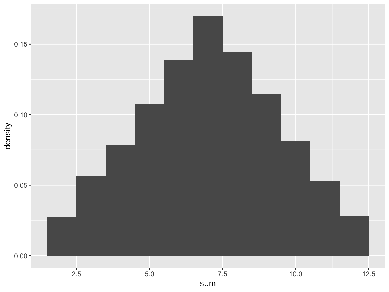
Figure 3.2: Histogram for Tossing Two Dice
It is often helpful to clarify a probability experiment and its sample space by making an artificial distinction. Pretend the dice are different colors, say, the first die white and the second die black. This allows us to distinguish between the individual outcomes on each die. Given that the six different outcomes on each side are equally likely, the resulting \(6 \cdot 6 = 36\) outcomes illustrated in the table below provides a sample space of equally likely outcomes from which to find the probability of events you are interested in.
Since there are 6 ways to roll the first white die and 6 ways to roll the second black die there are \(6 \cdot 6 = 36\) ways to roll both dice. This insight uses the Fundamental Counting Principle described below:
3.4 Fundamental Counting Principle
Consider a multi-step process requiring k steps. If Step1 can be done \(n_{1}\) ways, Step2 can be done $n_{2} ways, and so on up to Step k being done $n_{k} ways, then the total number of ways the entire process can be done \(n_{1} \cdot n_{2} \cdot ... \cdot n_{k}\) ways.
Furthermore, since all outcomes on each individual die are equally likely these 36 possibilities represent equally likely outcomes for the experiment of tossing two dice. We can use this sample space to answer some questions.
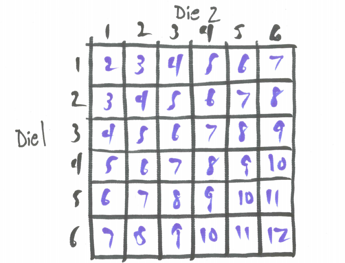
Figure 3.3: Sample Space for Two Dice
For example, there is only one combination of dice that yields a sum of 2 (that is 1+1) and there is only one combination of dice that yields a sum of 3 (that is 1+2) but a sum of 3 is twice as likely because when we distinguish the dice we see 1+2 and 2+1 as distinct options and we get \(P(sum=2)=1/36\) while \(P(sum=3)=2/36\).
Let’s try another one: which is more likely, a sum of 6 or a sum of 7? From the sample space we see five ways to obtain a 6 and six ways to obtain a 7 indicating a sum of 7 is more likely. Stated as probabilities, \(P(sum=6)=5/36\) and \(P(sum=7)=6/36\).
3.4.1 Practice
Which is more likely when tossing two dice, a sum of 3 or a sum of 11? Explain.
Simply by counting successes in the sample space we find the probability of compound events.
Let’s define a few events for this experiment of tossing two dice and find the probabilities of related compound events.
E: The sum is even. F: The sum is less than or equal to 5.
It is helpful to identify members of the sample space satisfying each event.
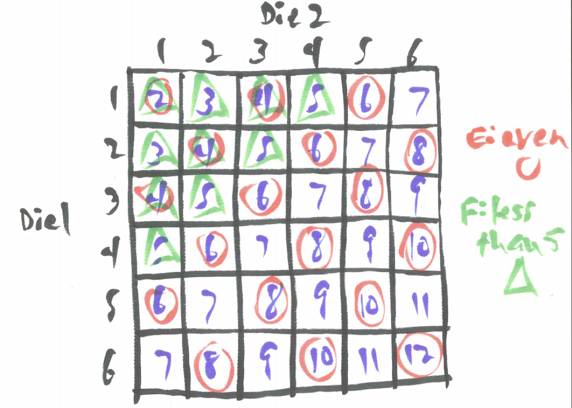
Figure 3.4: Sample Space for Two Dice with Events E and F
We see \(P(E)=18/36=1/2=0.5\) and also note \(P(not \ E)=18/36=1/2=0.5\). From the sample space, \(P(F)=10/36\) and \(P(not \ F)=26/36\).
Looking at compound events, recall that AND refers to the overlap where both events are true so \(P(E \ and \ F)=4/36\).
We think of OR as an inclusive or representing the event one or the other or both occur. Counting unique elements of the sample space that are either an even sum or a sum less than or equal to five we see \(P(E \ or \ F)=24/36\).
Conditional probability is trickier. \(P(E \mid F)\) means the probability that the sum is even given we know the sum is less than or equal to five. To handle this, we assume the sum is less than or equal to five and this narrows down our sample space to 10 possibilities of which 4 have an even sum yielding \(P(E \mid F)=4/10\).
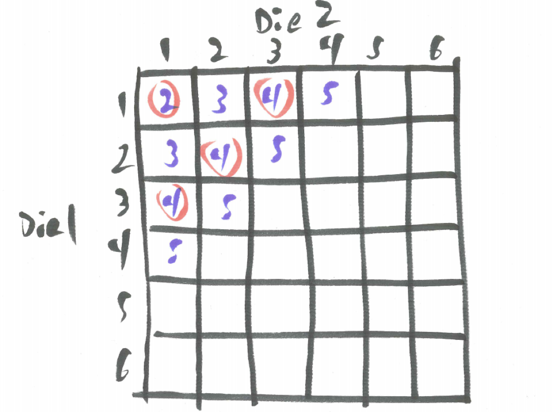
Figure 3.5: Sample Space for Two Dice Given F
It means something quite different to consider \(P(F \mid E)\), the probability the sum is less than or equal to five given it is even. Out of the 18 even sums, we find 4 of them are less than or equal to five yielding \(P(F \mid E)=4/18\).
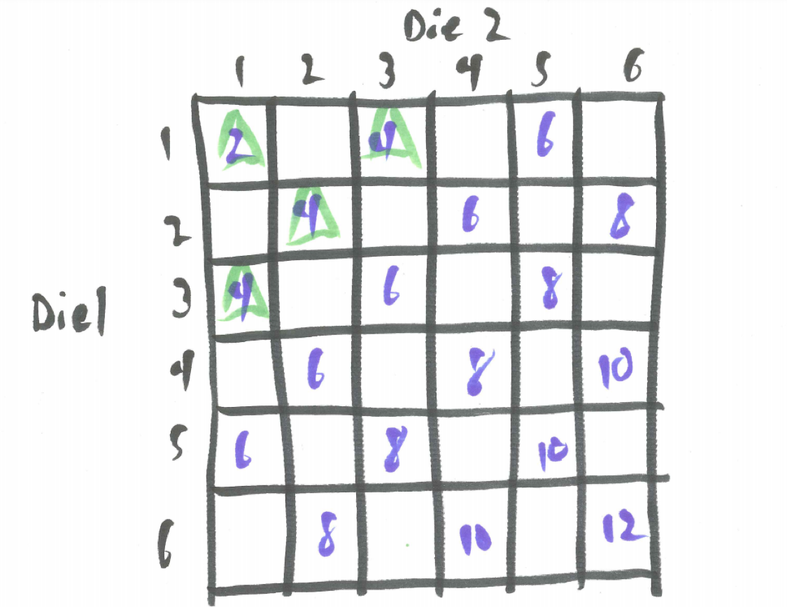
Figure 3.6: Sample Space for Two Dice Given E
It is important to note we found all of the probabilities above by focusing on the meaning of the events rather than some fancy formula.
3.5 Example - Galileo’s Dice Problem
In Galileo’s day, a clear understanding of probability was still being developed. While Galileo is well-known for his work on inventing the telescope and pointing it for the first time at the moon, his experimental approach to understanding the physics of motion dropping objects from the Tower of Pisa, and, most famously, his advocation of the Copernican planetary model and his subsequent condemnation by church authority, Galileo was also exploring the fundamental notions of chance.
The king approached Galileo for help with a mathematical problem. There was a gambling game involving tossing three dice. According to conventional reasoning a sum of nine should occur with the same frequency as a sum of ten because there were an equal number of ways to obtain each. There were six dice combinations to obtain a sum of 9 - 1+2+6, 1+3+5, 1+4+4, 2+2+5, 2+3+4, and 3+3+3. Similarly, there were six dice combinations to obtain a sum of 10 - 1+3+6, 1+4+5, 2+2+6, 2+3+5, 2+4+4, and 3+3+4.
However, it had been observed that a sum of ten occurred more frequently than a sum of nine. While not thrilled to divert his attention to solving the king’s problems, Galileo nevertheless looked into the issue and thereby advanced the theory of probability. We can walk in Galileo’s footsteps and discover why the theory of the time and the real-world experience did not agree?
To see how Galileo solved this problem we need to absorb the lesson of creating a helpful artificial distinction. Let’s pretend we can tell the dice apart.
First of all, since there are 6 equally likely outcomes on each die, there are \(6 \cdot 6 \cdot 6=216\) total equally likely outcomes in the sample space.
Let’s examine the different combinations of 9 and 10 in the light of distinguishable dice where order matters.
Sum of Nine
- Combo 1+2+6 - Orderings 1+2+6, 1+6+2, 2+1+6, 2+6+1, 6+1+2, 6+2+1
- Combo 1+3+5 - Orderings 1+3+5, 1+5+3, 3+1+5, 3+5+1, 5+1+3, 5+3+1
- Combo 1+4+4 - Orderings 1+4+4, 4+1+4, 4+4+1
- Combo 2+2+5 - Orderings 2+2+5, 2+5+2, 5+2+2
- Combo 2+3+4 - Orderings 2+3+4, 2+4+3, 3+2+4, 3+4+2, 4+2+3, 4+3+2
- Combo 3+3+3 - Orderings 3+3+3
Sum of Ten
- Combo 1+3+6 - Orderings 1+3+6, 1+6+3, 3+1+6, 3+6+1, 6+1+3, 6+3+1
- Combo 1+4+5 - Orderings 1+4+5, 1+5+4, 4+1+5, 4+5+1, 5+1+4, 5+4+1
- Combo 2+2+6 - Orderings 2+2+6, 2+6+2, 6+2+2
- Combo 2+3+5 - Orderings 2+3+5, 2+5+3, 3+2+5, 3+5+2, 5+2+3, 5+3+2
- Combo 2+4+4 - Orderings 2+4+4, 4+2+4, 4+4+2
- Combo 3+3+4 - Orderings 3+3+4, 3+4+3, 4+3+3
Tallying the orderings we see there are 25 orderings yielding a sum of 9 and 27 yielding a sum of 10 thus \(P(sum=9)=25/216=0.116\) while \(P(sum=10)=27/216=0.125\) confirming the real-world experience that a sum of 10 is actually more likely than a sum of 9.
A simulation might reinforce this. We simulate the sum of 10,000 tosses of three dice and examine the frequency table of results.
die1 <- sample(x=1:6, size=10000, replace = TRUE)
die2 <- sample(x=1:6, size=10000, replace = TRUE)
die3 <- sample(x=1:6, size=10000, replace = TRUE)
sum3 <- die1 + die2 + die3
sim_three_dice <- data.frame(die1, die2, die3, sum3)
knitr::kable(
  table(sum3), caption = 'Tossing Three Dice Simulation',
  booktabs = TRUE
)| sum3 | Freq |
|---|---|
| 3 | 45 |
| 4 | 136 |
| 5 | 277 |
| 6 | 451 |
| 7 | 704 |
| 8 | 971 |
| 9 | 1156 |
| 10 | 1197 |
| 11 | 1301 |
| 12 | 1159 |
| 13 | 960 |
| 14 | 688 |
| 15 | 455 |
| 16 | 270 |
| 17 | 178 |
| 18 | 52 |
We can examine the relative frequencies.
knitr::kable(
  prop.table(table(sum3)), caption = 'Relative Frequencies for Tossing Three Dice Simulation',
  booktabs = TRUE
)| sum3 | Freq |
|---|---|
| 3 | 0.0045 |
| 4 | 0.0136 |
| 5 | 0.0277 |
| 6 | 0.0451 |
| 7 | 0.0704 |
| 8 | 0.0971 |
| 9 | 0.1156 |
| 10 | 0.1197 |
| 11 | 0.1301 |
| 12 | 0.1159 |
| 13 | 0.0960 |
| 14 | 0.0688 |
| 15 | 0.0455 |
| 16 | 0.0270 |
| 17 | 0.0178 |
| 18 | 0.0052 |
Are the relative frequencies for obtaining a sum of 9 and for obtaining a sum of 10 similar to what theory suggests?
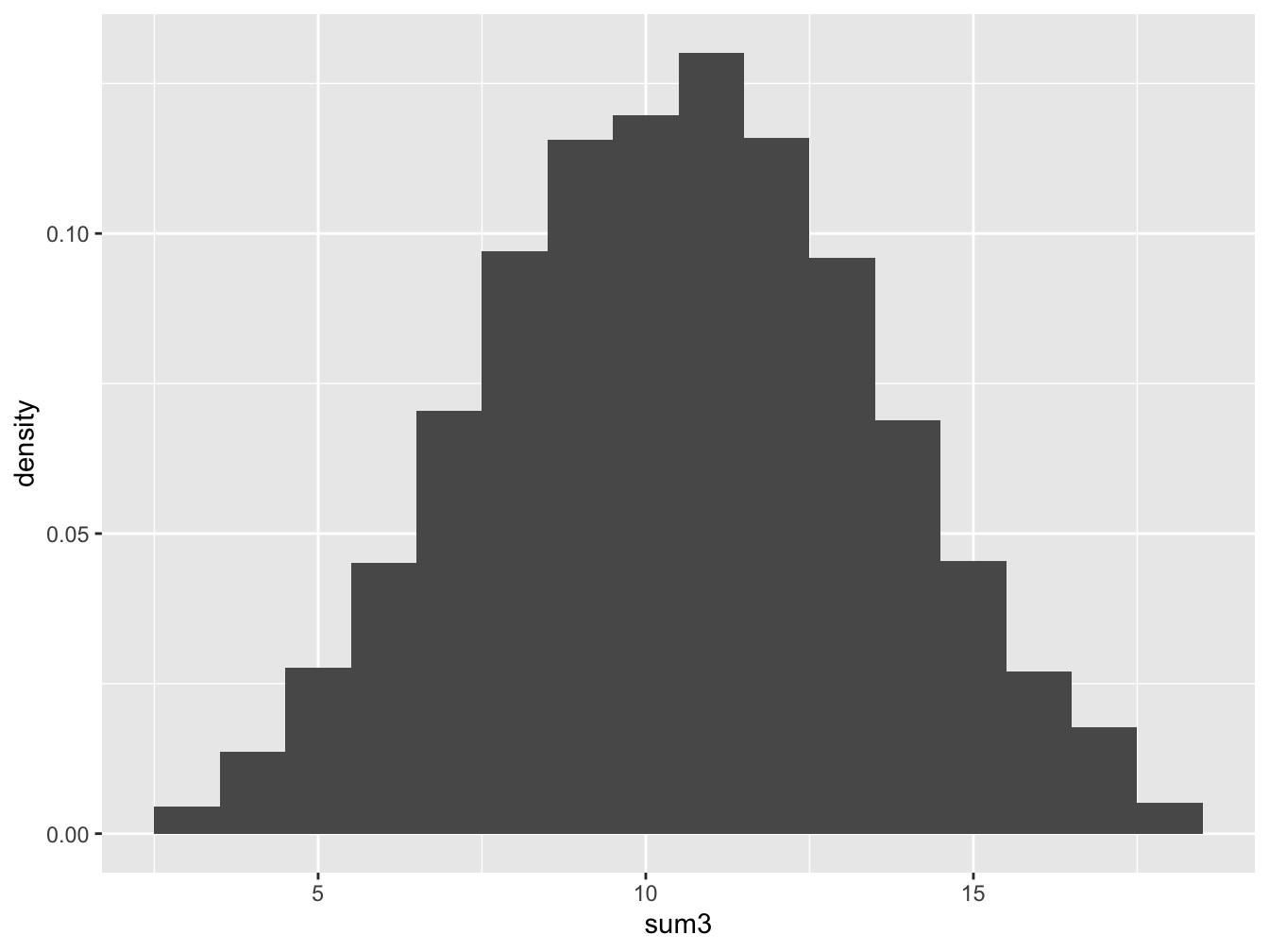
Figure 3.7: Histogram for Tossing Three Dice
Although the difference is small, attentive human eyes observed it and persistent inquiring minds found the theory needed to explain it. This is often the way knowledge develops - from careful observation about in the world to an explanatory mathematical model.
3.6 Chapter Scenario Revisited - The Game of Diff
In the Game of Diff the player pays a certain fee and then rolls two dice and wins in dollars the difference. We can run an R simulation tossing two dice and computing the difference a large number of times to get a better sense of expected winnings.
# Simulate 10000 die tosses and the difference and put in a data frame
die1 <- sample(1:6, 10000, replace=TRUE)
die2 <- sample(1:6, 10000, replace=TRUE)
diff <- abs(die1 - die2)
diff_data <- data.frame(die1, die2, diff)
head(diff_data)
## die1 die2 diff
## 1 4 6 2
## 2 3 1 2
## 3 2 3 1
## 4 6 1 5
## 5 2 3 1
## 6 2 5 3We tabulate the simulation results with a frequency table and a relative frequency table.
##
##    0    1    2    3    4    5
## 1639 2793 2216 1726 1102 524##
## 0 1 2 3 4 5
## 0.1639 0.2793 0.2216 0.1726 0.1102 0.0524We can visualize the differences with a histogram.
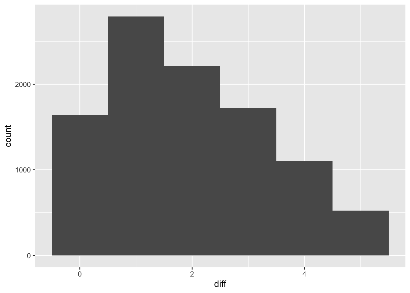
What was the most common difference? What was the least common difference? Computing summary statistics provides important information.
##  min Q1 median Q3 max   mean       sd     n missing
##    0  1      2  3   5 1.9431 1.420163 10000       0
The mean difference based on the simulation of 10,000 trials is 1.9431. How do these results compare with theory. Now, we find the mean value for the Game of Diff using our traditional, theoretical analysis.
With two dice being tossed we want to start with the sample space of the 36 equally likely outcomes. We complete the table by identifying the value of the difference over these outcomes.
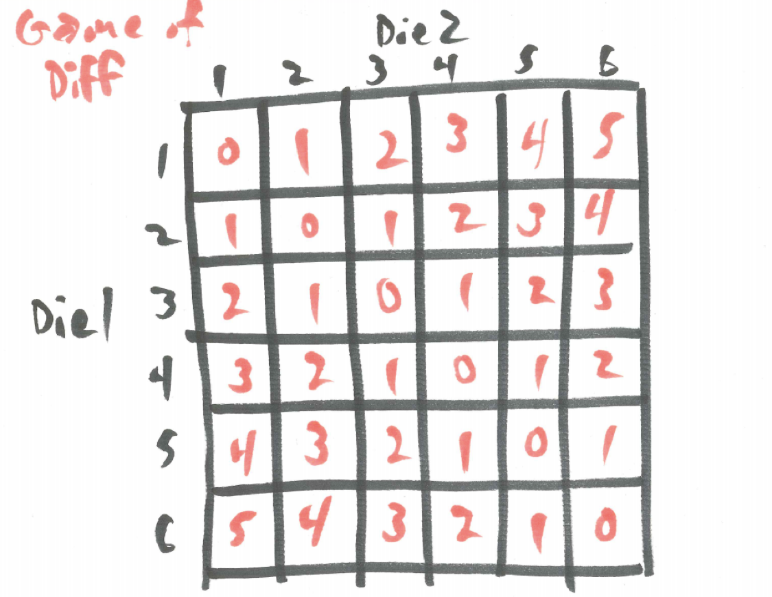
Figure 3.8: Table for the Difference of Two Dice
By counting the number of occurrences of each possible difference we find the probability distribution for X, the difference of two dice.
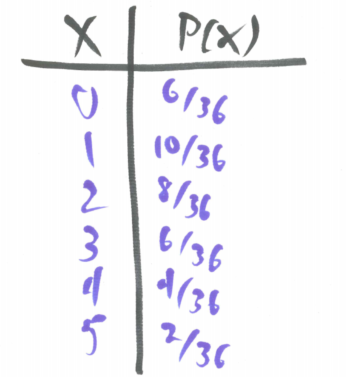
Figure 3.9: Probability Distribution for the Difference of Two Dice
Based on the table, we can find and input the probability distribution and compute the mean/expected value using R.
x <- c(0, 1, 2, 3, 4, 5)
probs <- c(6/36, 10/36, 8/36, 6/36, 4/36, 2/36)
expectation_diff <- sum(x*probs)
expectation_diff
## [1] 1.944444The true expected value for the game of diff is 1.9444444. How close was the sample mean generated from simulation to the true mean found by the expected value formula? We know, in the long run, the sample mean will approach the true, theoretical expected value.
Accordingly, based on the simulation results and theoretical results above, what you would now recommend for the price of the game including how much money you would predict the casino would make per game and the house advantage as a percentage. Of course, you need to balance two things. First, you want to make sure you set a price that is greater than the expected value to ensure profitibility for the casino. Second, you want to the price to be competitive and still attract gamblers. What price would you recommend?
3.7 Exercises
3.7.1 Exercise - My Die, Your Die
Suppose that I toss a die and you toss a die. Find the probability of the following events. (a) Your die is the same result as my die. (b) Your die is different than my die. (c) Your die is greater than my die.
3.7.2 Exercise - Three Dice
Three dice are tossed. Answer the following questions. (a) Which is more likely - rolling a sum of 3 or a sum of 18? (b) Which is more likely - rolling a sum of 4 or a sum of 17? (c) Which is more likely - rolling a sum of 10 or a sum of 11? (d) Which is more likely - rolling a sum of 10 or less or rolling a sum of 11 or more?
3.7.3 Exercise - Dice Games
Consider the two-person dice games described below. For each game determine which player has an advantage or whether the two options are equally likely. (a) In Game One, two dice are rolled and Asmah wins if the sum is odd and Ismail wins if the sum is even. (b) In Game Two, two dice are rolled and Asmah wins with a sum of 2,3,4,5,10,11,12 and the Ismail wins with a sum of 6,7,8,9.
3.7.4 Exercise - De Morgan’s Laws
The negation of “A or B” is “not A and not B”. The negation of “A and B” is “not A or not B”. These logical observatons are called De Morgan’s Laws. For the event of tossing two dice with A being the event of rolling doubles and B being the event of rolling a sum of seven, describe the following events verbally and find their probability. (a) not(A or B) (b) not(A and B)